Project 1: Lightfield Camera
Overview
Prof. Ren Ng et al. demonstrated that capturing images over a plane orthogonal to the optical axis (for example, along the image/sensor plane) allows one to create complex effects using very simple processing. These images of the same scene captured from different angles of view allow for post-capture refocusing and aperture resizing. Having lightfield data is especially useful for photographers because they no longer have to trade off controlling depth of field to control motion blur, and vice versa. My goal was to recreate these effects using real lightfield data.
I used the rectified images provided in the Stanford Light Field Archive, which has sample datasets comprising of multiple images taken over a regularly spaced grid. I use alignment and averaging methods to implement depth refocusing and aperture adjustment on the sample data.
Note: if the GIFs don’t play properly, reload or open the GIF in a new tab.
Part 1.1: Depth Refocusing
The objects which are far away from the camera do not vary their position significantly when the camera moves around while keeping the optical axis direction unchanged. The nearby objects, on the other hand, vary their position significantly across images. Averaging all the images in the grid without any shifting will produce an image which is sharp around the far-away objects but blurry around the nearby ones. Similarly, shifting the images “appropriately” and then averaging allows one to focus on object at different depths.
Each sub-aperture image in the Stanford dataset can be seen as the light from a different part of a “universal aperture” (or the same “back of the lens” picture taken many times from slightly different positions). These images can be thought of as light rays because each (x, y) position on the image plane and (u, v) position on the aperture plane uniquely define a ray. In the dataset, the (x, y) is fixed while (u, v) is varied. This gives us a set of rays that will be integrated by a single point on the image plane, which we repeat for every point on the image plane.
Using this idea, I implement a function to generate images focusing on different depths. After extracting sub-aperture positional information by parsing the filenames of images in the dataset, I determined the position of the center microlens. Since the Stanford Light Field Archive datasets I used have a 17x17 microlens array, I used (8, 8) as the center. I then implemented my depth refocusing algorithm as follows (with guidance from past lecture slides):
- For each sub-aperture image I(x, y):
- Calculate the displacement (u, v) from the center.
- Shift the sub-aperture image by C * (u, v), where C is an arbitrary scaling factor. If shifts are not integers, bilinear interpolation may be needed.
- Average all of the shifted images.
Note that a larger C means refocusing further from the physical focus, and the sign of C affects whether we are focusing closer or further.
I initially used np.roll to actually shift the image, but I switched to scipy.ndimage.shift so allow for non-integer shifts when using fractional values of C. Because of system limitations and image sizes, I used order = 1 (linear) as the interpolation parameter because the visual difference between images interpolated at order = 1 and order = 3 was very minimal, with an ~8x speedup.


The same image interpolated using order 0, 1, 2, and 3. The significant performance improvement justifies the *slight*, hardly noticeable decrease in interpolation quality.
Here are my results on different datasets:
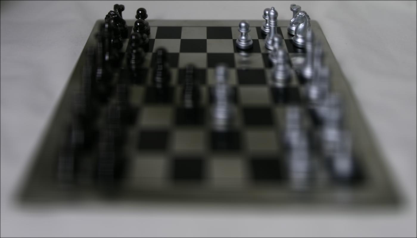
Chess; generated with evenly spaced C = -0.5 to 3.0
Eucalpytus flowers; generated with evenly spaced C = -0.5 to 3.0
Amethyst; generated with evenly spaced C = -1.5 to 3.0
Lego Bulldozer; generated with evenly spaced C = -1.5 to 3.0
Part 1.2: Aperture Adjustment
Averaging a large number of images sampled over the grid perpendicular to the optical axis mimics a camera with a much larger aperture, and using fewer images results in an image that mimics a smaller aperture.
To change the aperture, I modified my shift function to add an aperture threshold in order to reduce the number of images we use in our averaging, and also to reduce the shift of the images we do choose to include. The aperture threshold sets the maximum radius from the center that we will include in our average image. If the threshold is large, we’d average over many images and create a larger aperture, or a shallow depth of field.
A brief note about noise: having more sub-aperture images in the result may introduce more noise/blur because of the distance between sub-apertures and their slight difference in views.
Here are my results on different datasets. For all results, I use an aperture thresholds from 0 to 10, incrementing by 1 for each image. The value of C is held constant across these images and is specified in the caption of each output.
Chess; C = 1.0
Eucalpytus flowers; C = 2.5

Amethyst; C = 0.8
Lego Bulldozer; C = 2.5
Crystal Ball; C = 0.1
Part 1.3: Summary
I was impressed by how the simple idea of placing multiple sensors, combined with elementary operations, can lead to really interesting results. I looked up more information about the Lytro camera (R.I.P.) and it made me interested in actually getting on to experiment. I learned a lot about computational photography through this project, and definitely feel like I have a better grasp on how to manipulate rays and the nuances of depth focusing and aperture. If I had more time, I would’ve tried to set up my own setup to take photos simulating different rays in the same scene to try to create my own dataset.
Project 2: High Dynamic Range Imaging
Overview
Modern cameras are unable to capture the full dynamic range of commonly encountered real-world scenes. In some scenes, even the best possible photograph will be partially under or over-exposed. Researchers and photographers commonly get around this limitation by combining information from multiple exposures of the same scene. In this project, using starter code from Brown and methods described in Debevec and Malik 1997 and Durand 2002, I implement tools to automatically combine multiple exposures into a single high dynamic range radiance map, and then convert this radiance map to an image suitable for display through tone mapping.
Part 2.1: Radiance Map Construction
The observed pixel value \(Z_{ij}\) for pixel i in image j is a function of unknown scene radiance and known exposure duration: \(Z_{ij} = f(E_i \Delta t_j)\). \(E_i\) is the unknown scene radiance at pixel i, and scene radiance integrated over some time \(E_i Δt_j\) is the exposure at a given pixel.
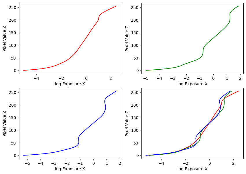
In general, \(f\) might be a somewhat complicated pixel response curve. We will not solve for \(f\), but for \(g=ln(f^{-1})\) which maps from pixel values (0-255) to the log of exposure values: \(g(Z_{ij}) = ln(E_i) + ln(t_j)\) (equation 2 in Debevec). Solving for g might seem impossible (we only recover g up to a scale factor) because we know neither \(g\) or \(E_i\). The key observation is that the scene is static, and while we might not know the absolute value of \(E_i\) at each pixel i, we know these values must be constant.
To solve for \(g\), we impose some constraints then construct and solve a system of linear equations using least squares. First, we assume \(g\) is smooth and monotonic, so we can add a constraint to penalize its second derivative term. We can construct this second derivative using finite differences: \(g'' = \left(g(x - 1) - g(x)\right) - \left(g(x) - g(x + 1)\right) = g(x - 1) + g(x + 1) - 2 \cdot g(x)\).
To motivate \(g\) to be smooth, we add a regularizing constraint of the form: \(\lambda \left[ g(x - 1) w(x - 1) + g(x + 1) x(i + 1) - 2 g(x) w(x) \right] = 0\)
Finally, we solve for \(g\) in the overdetermined problem using least squares.
Then, to compute the radiance map for each pixel and using a weighting function to get better results, we follow equation 6 in Debevec:
\(\ln E_i = \frac{\sum_{j=1}^P w(Z_{ij}) \left(g(Z_{ij}) - \ln \Delta t_j \right)}{\sum_{j=1}^P w(Z_{ij})}\)
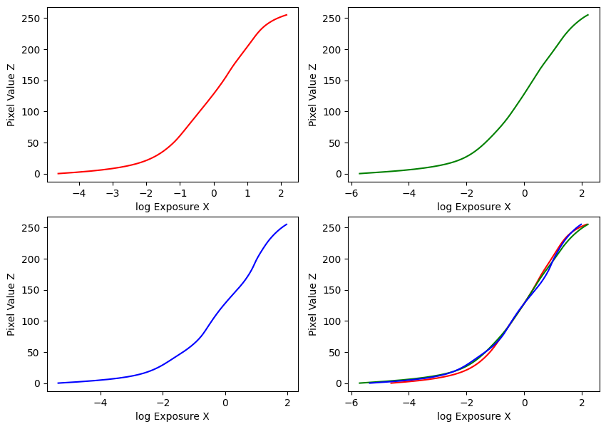
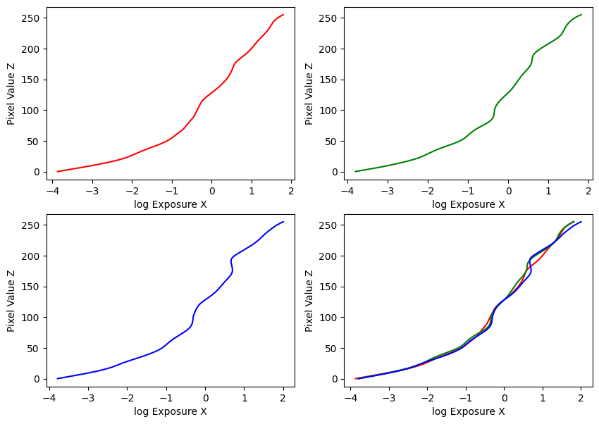
My implementation was guided by these methods in the paper, and the provided Matlab implementation in Appendix A. Using the provided datasets, my estimated g and recovered radiance maps are below:
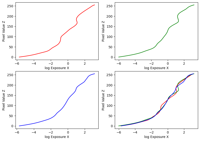
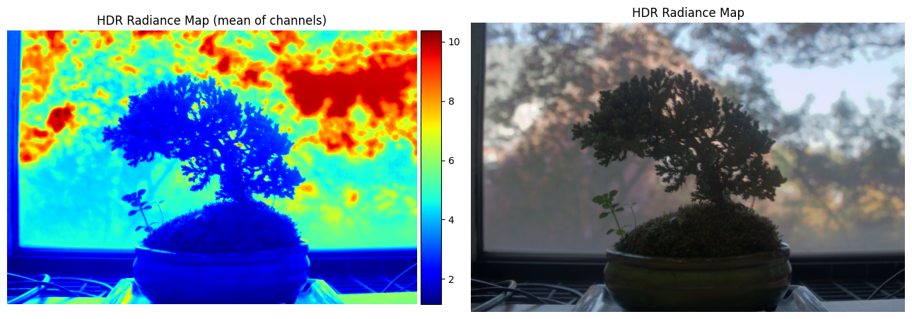
Estimated g and recovered radiance map for bonsai
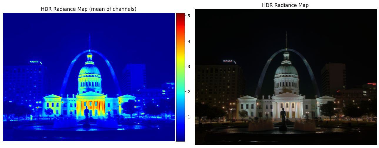
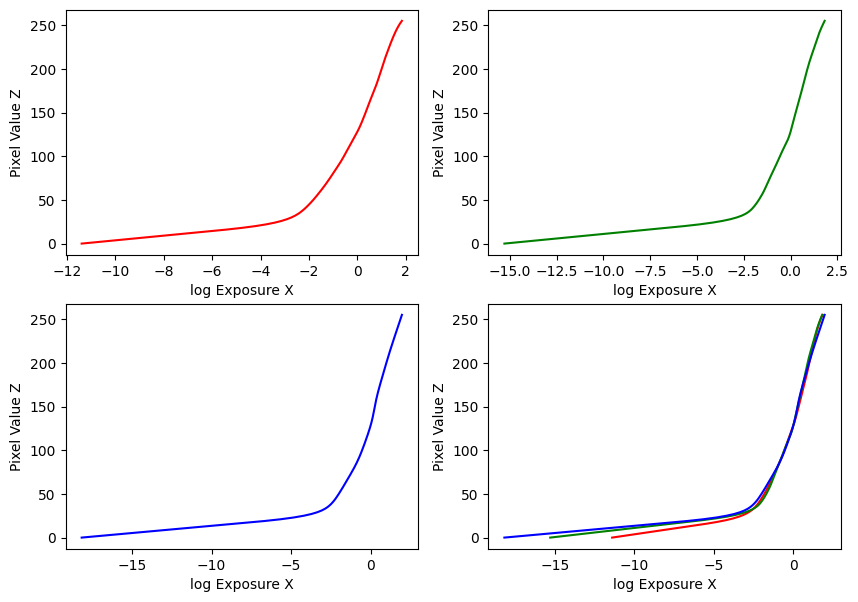
Estimated g and recovered radiance map for arch
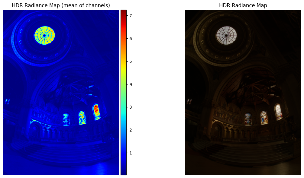
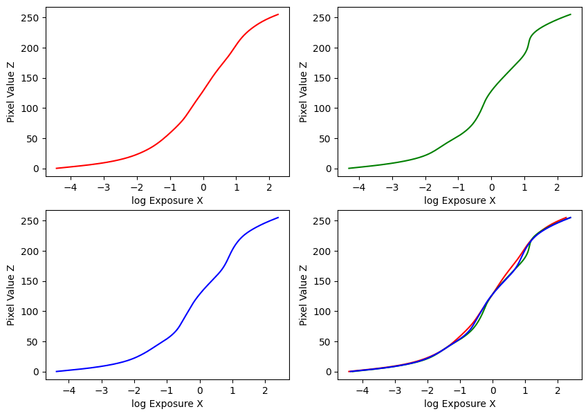
Estimated g and recovered radiance map for chapel
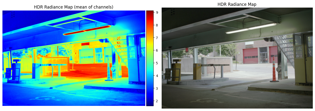
Estimated g and recovered radiance map for garage
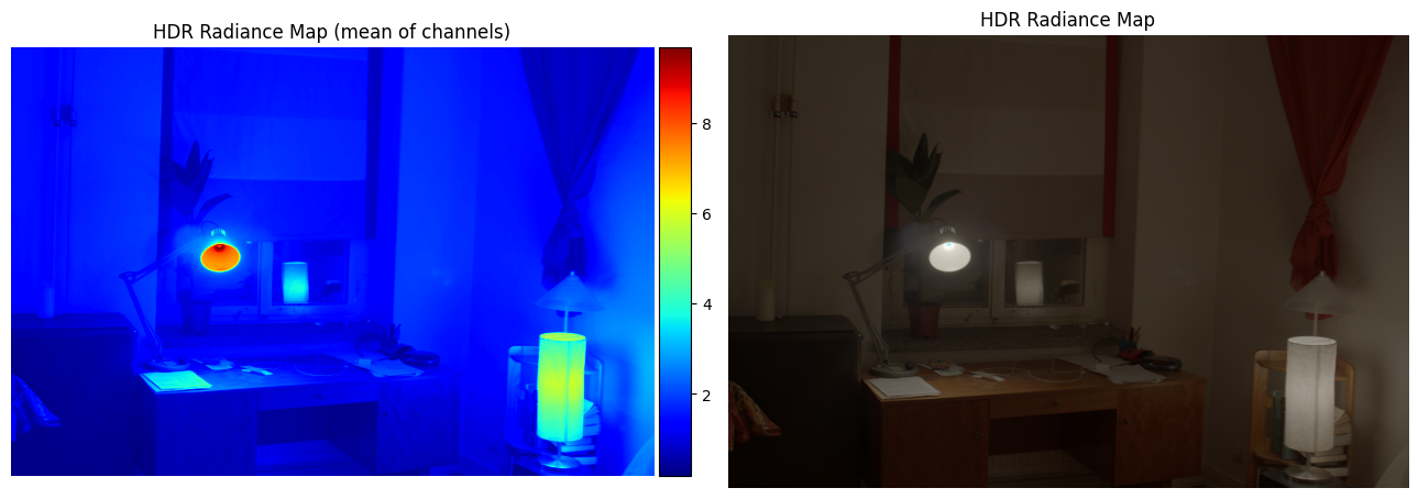
Estimated g and recovered radiance map for window
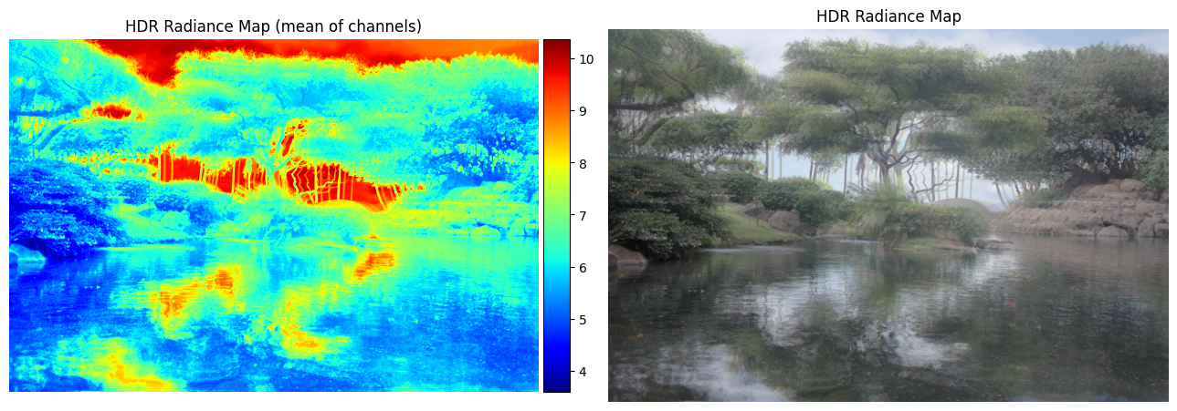
Estimated g and recovered radiance map for garden
Part 2.2: Tone Mapping
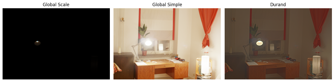
First, I implemented a simple global tone-mapping method following \(E_{display} = E_{world} / (1 + E_{world})\), where \(E_{world}\) is just the HDR radiance map.
Then, I implemented a local tone-mapping method following Durand 2002, to provide a more satisfying result. The algorithm is as follows:
- Your input is linear RGB values of radiance.
- Compute the intensity \(I\) by averaging the color channels.
- Compute the chrominance channels: \((\frac{R}I,\frac{G}I, \frac{B}I)\)
- Compute the log intensity: \(L = log_2(I)\) and add a small value to prevent zeroes causing instability issues.
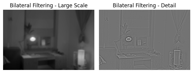
- Filter that with a bilateral filter: \(B = bilateralfilter(L)\)
- Compute the detail layer: \(D = L - B\)
- Apply an offset and a scale to the base: \(B' = (B - o) * s\)
- The offset is such that the maximum intensity of the base is 1. Since the values are in the log domain, \(o = max(B)\).
- The scale is set so that the output base has dR stops of dynamic range, i.e., \(s = dR / (max(B) - min(B))\).
- Reconstruct the log intensity: \(O = 2^{(B' + D)}\)
- Put back the colors: \(R',G',B' = O * (\frac{R}I,\frac{G}I, \frac{B}I)\)
- Apply gamma compression, otherwise the result will look too dark.
I used dr = 5, and gamma = 0.5.
My results are below:
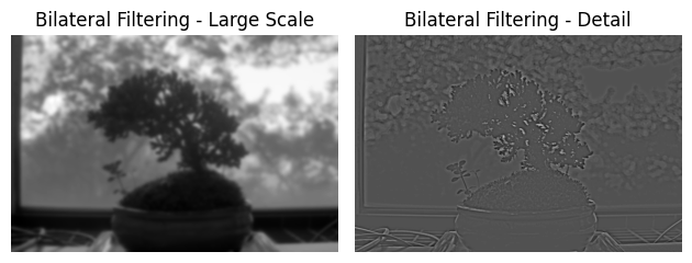
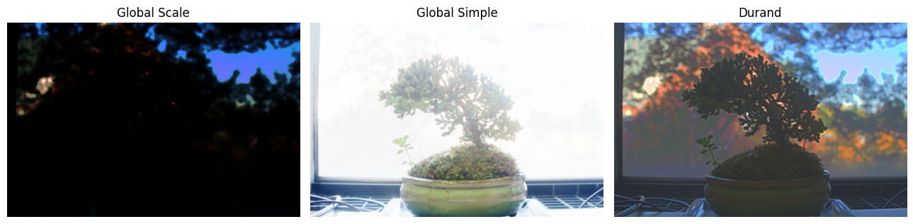
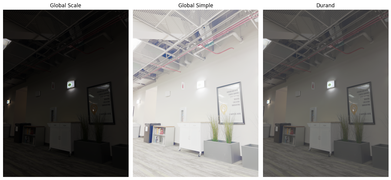
Bilateral filtering results and comparison of the three tone mapping methods for bonsai
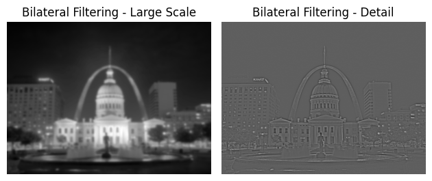

Bilateral filtering results and comparison of the three tone mapping methods for arch
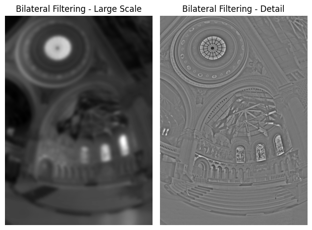
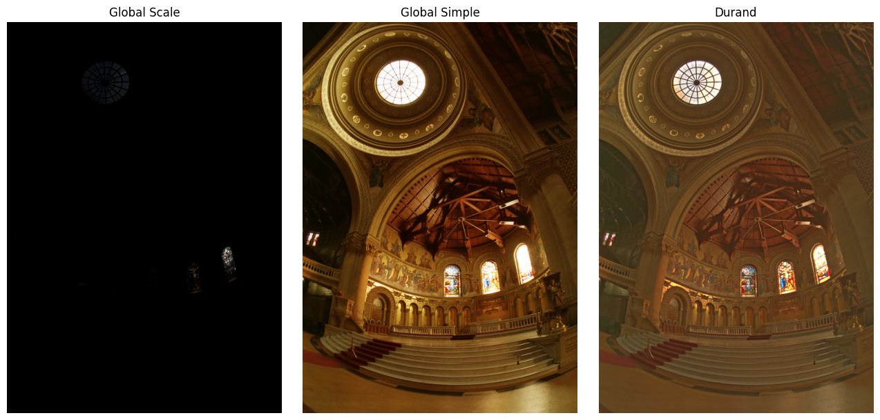
Bilateral filtering results and comparison of the three tone mapping methods for chapel
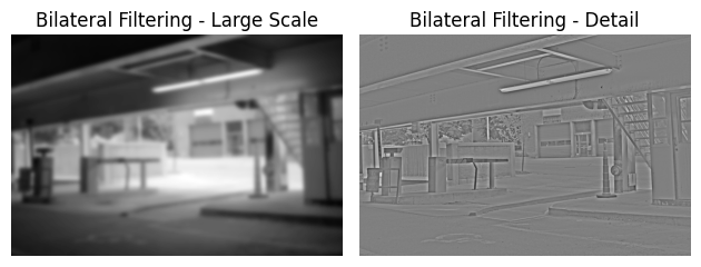
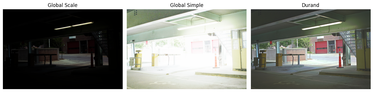
Bilateral filtering results and comparison of the three tone mapping methods for garage
Bilateral filtering results and comparison of the three tone mapping methods for window
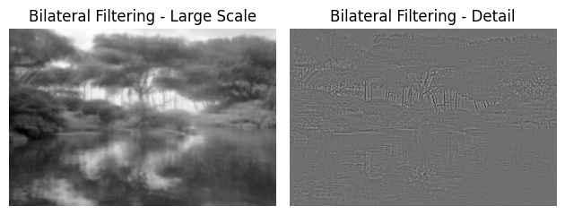
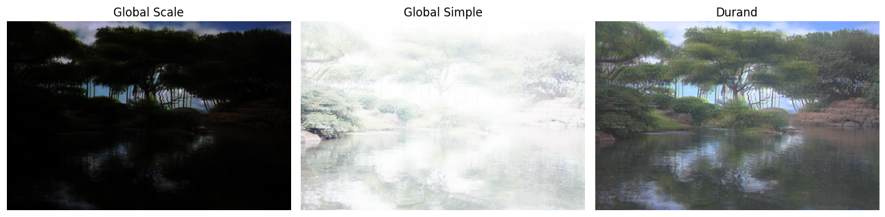
Bilateral filtering results and comparison of the three tone mapping methods for garden
Bells and Whistles
After a LOT of attempts to capture adequate sets of images with different exposures, I managed to create 3 of my own image sets and ran the algorithm on my own images. After creating a stable camera setup for each scene, I captured several images at different exposure levels, and recovered the exposure times from image metadata. My results are below:
Image Set #1: Wall
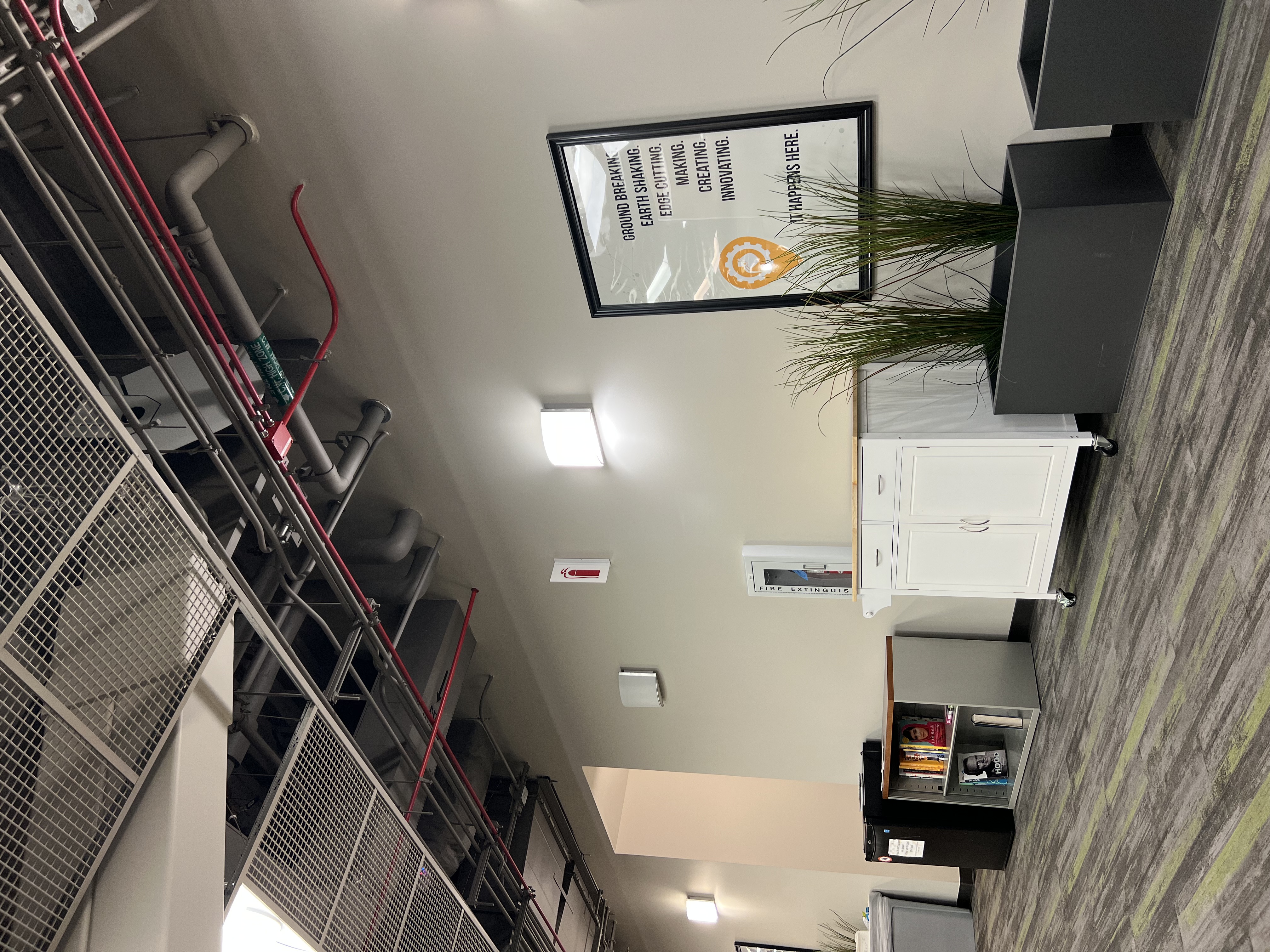
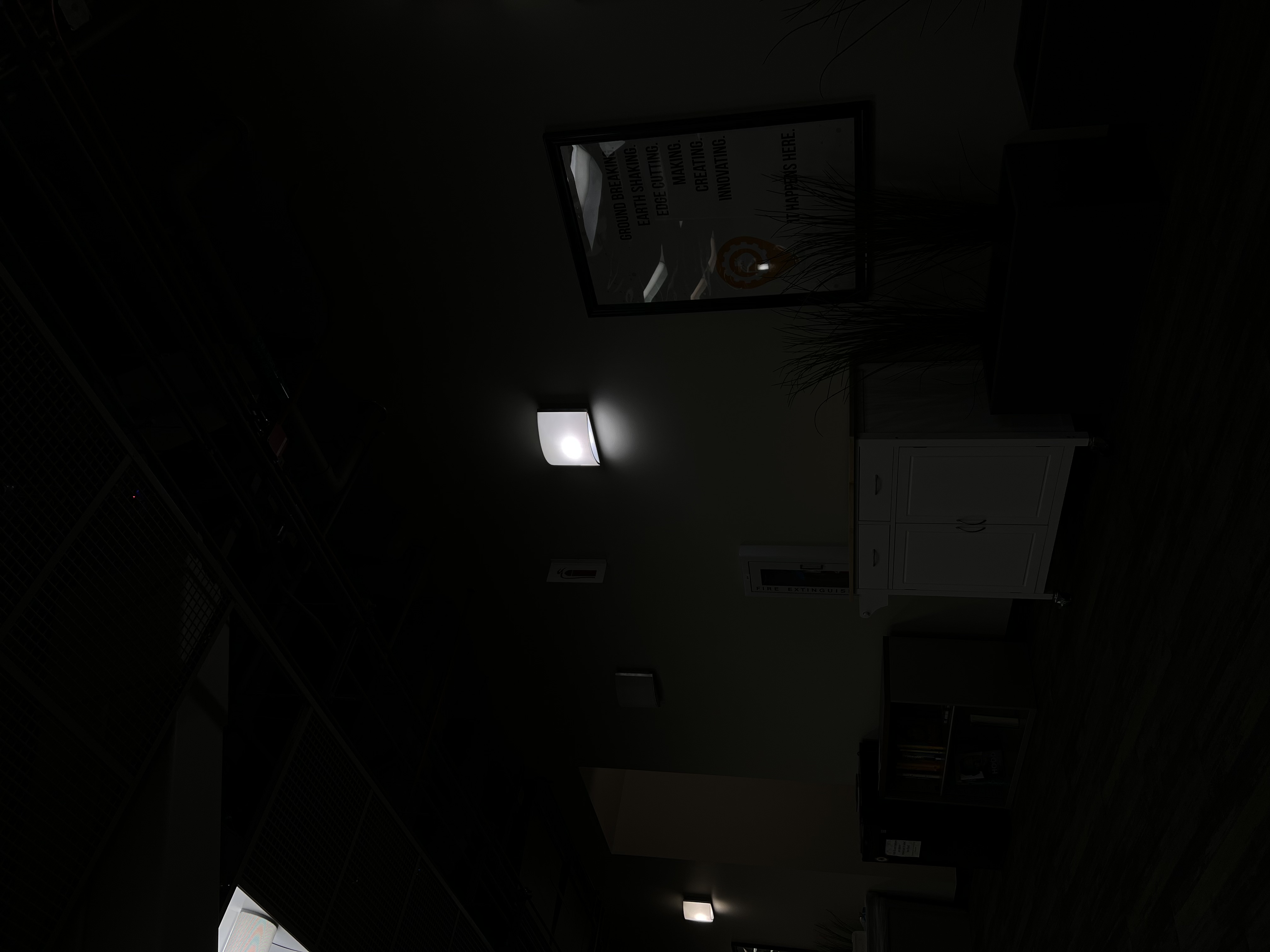
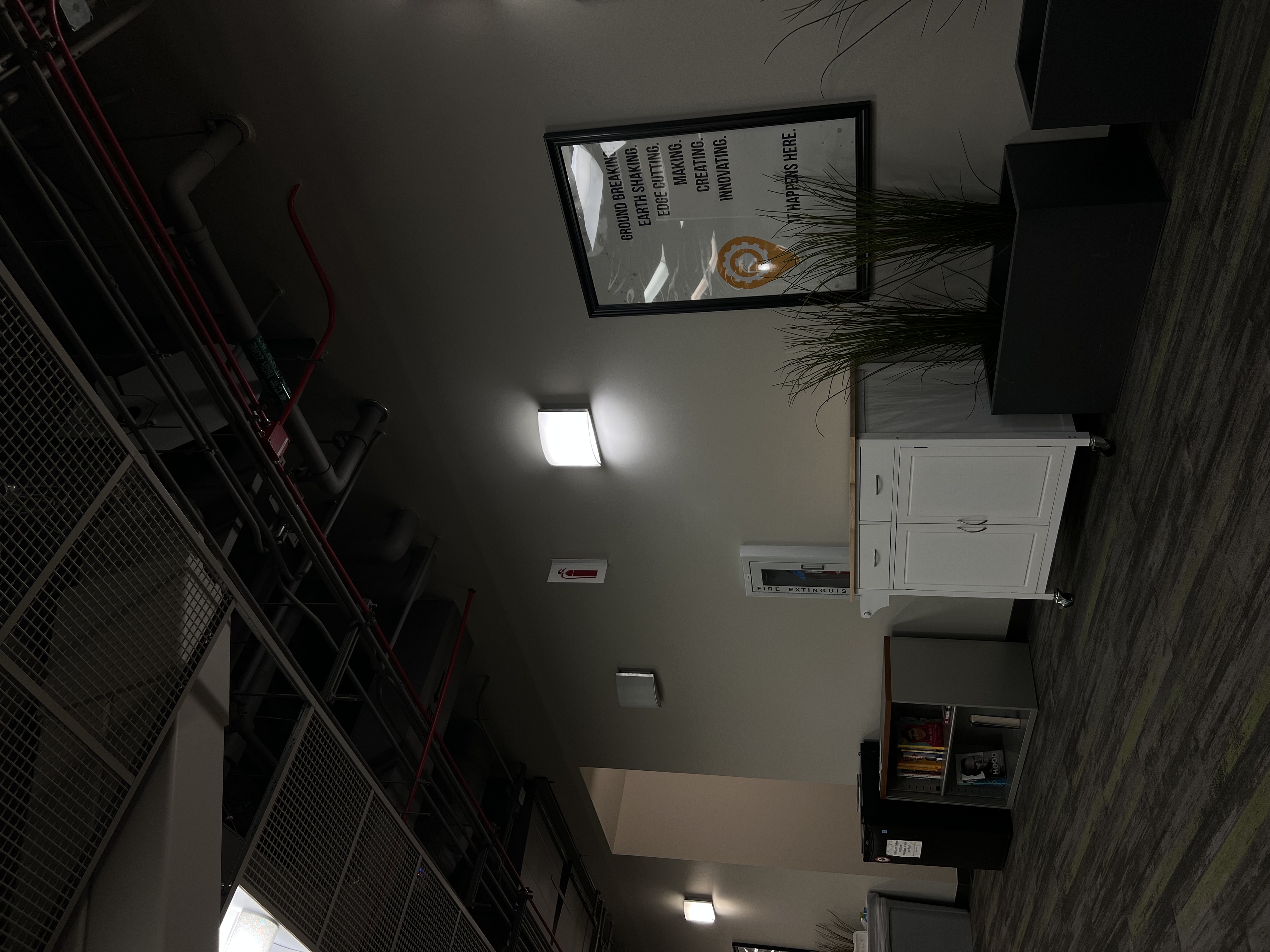
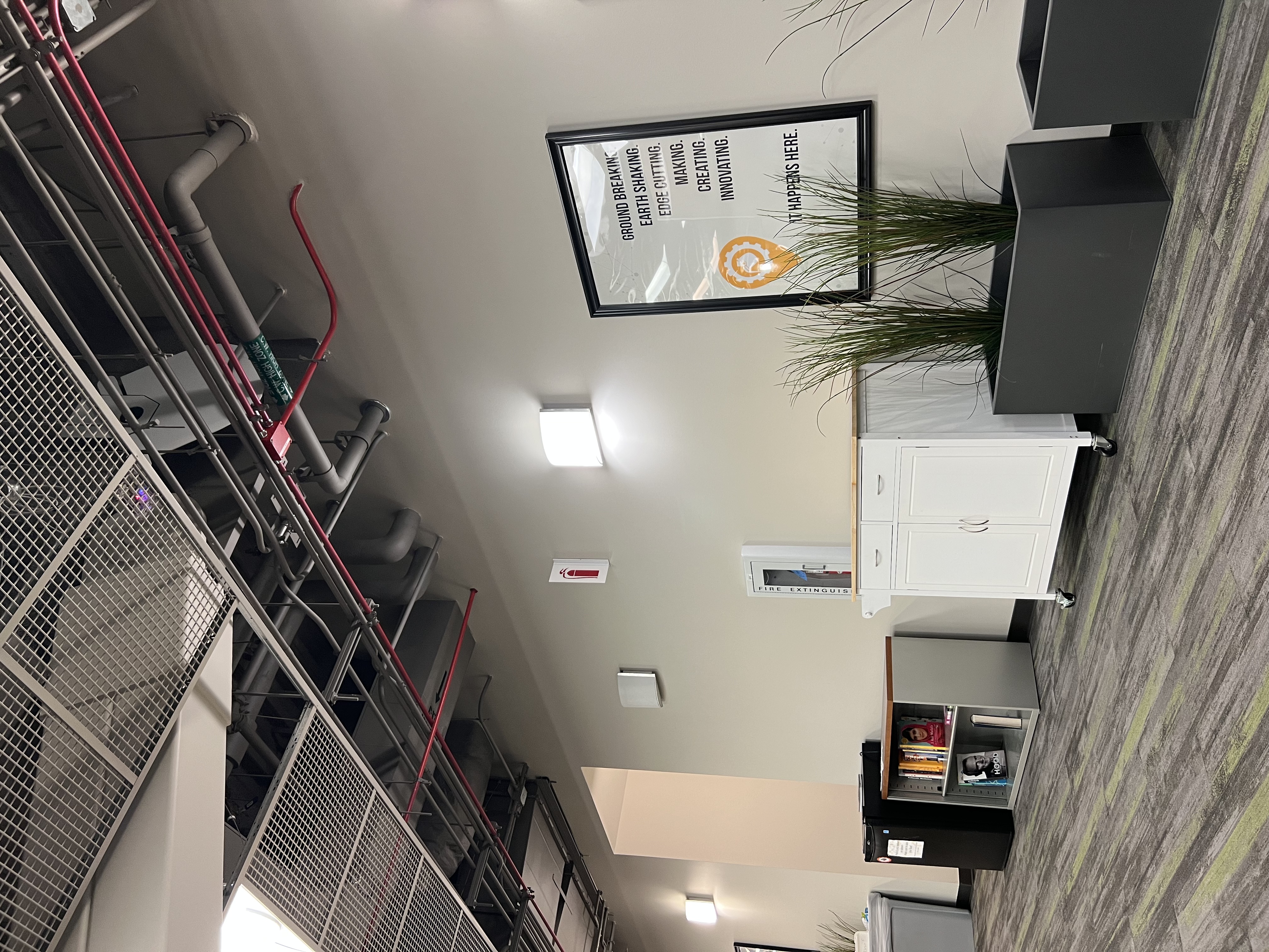
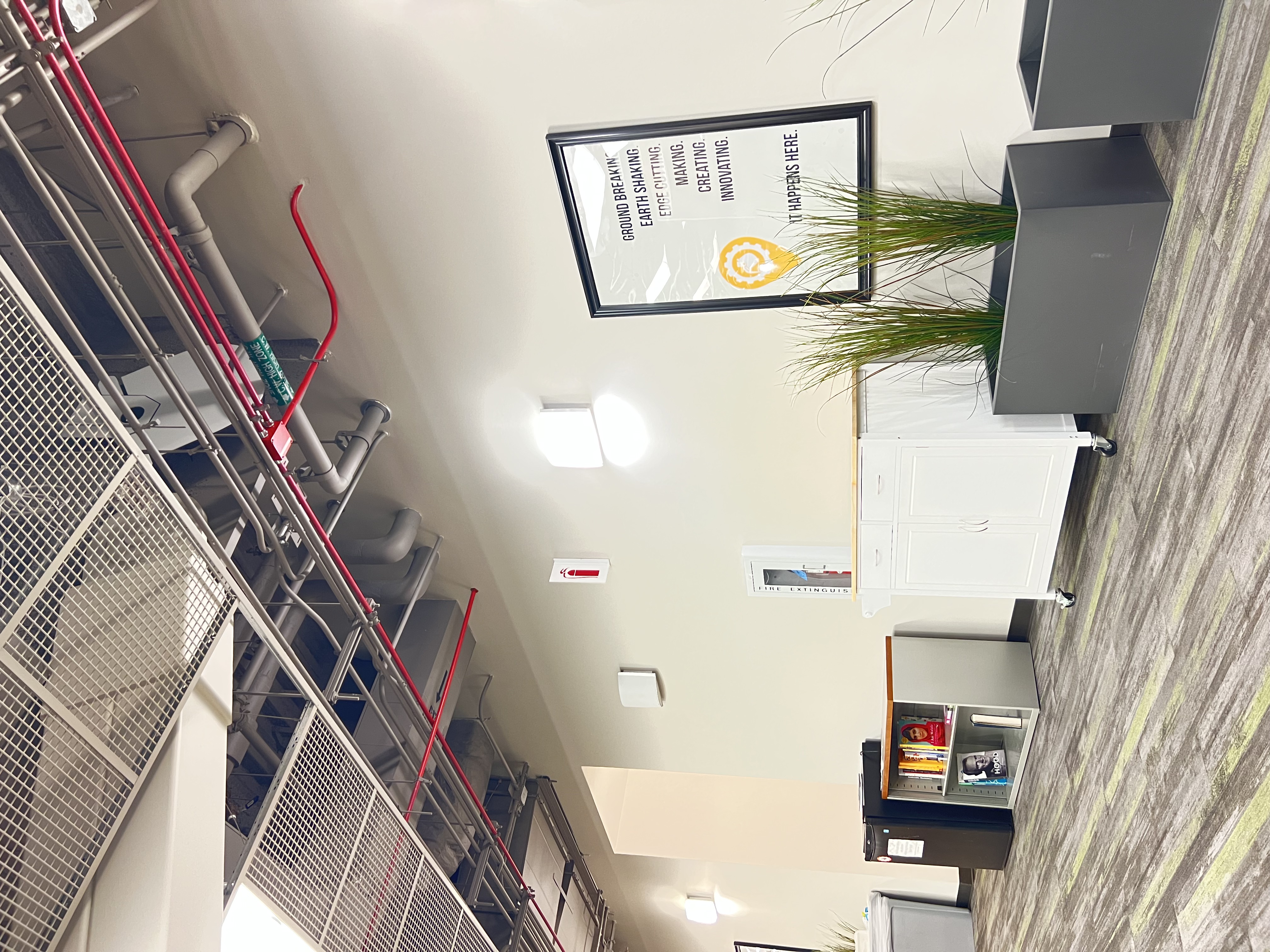
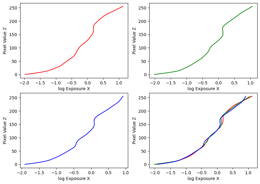
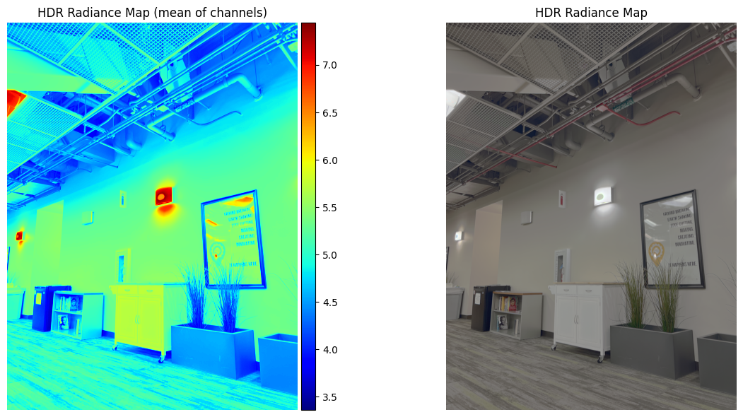
Estimated g and recovered radiance map for wall
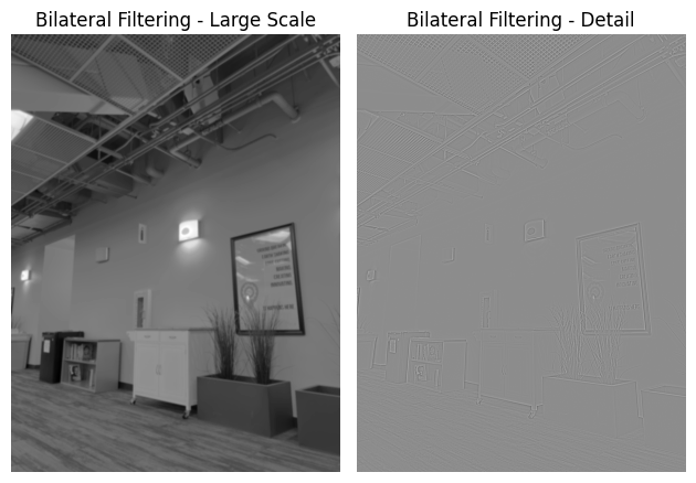
Bilateral filtering results and comparison of the three tone mapping methods for wall
Image Set #2: Sunset
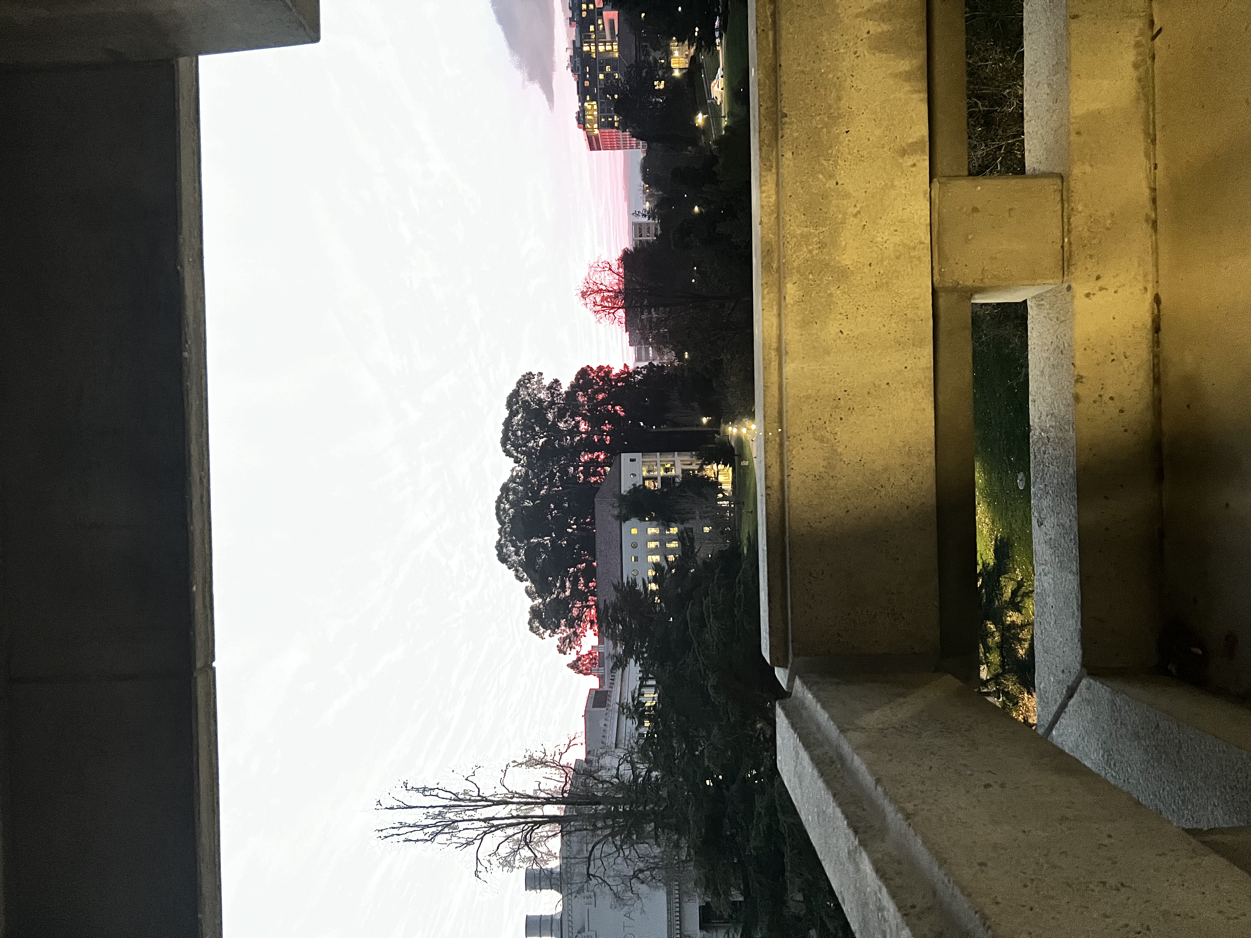
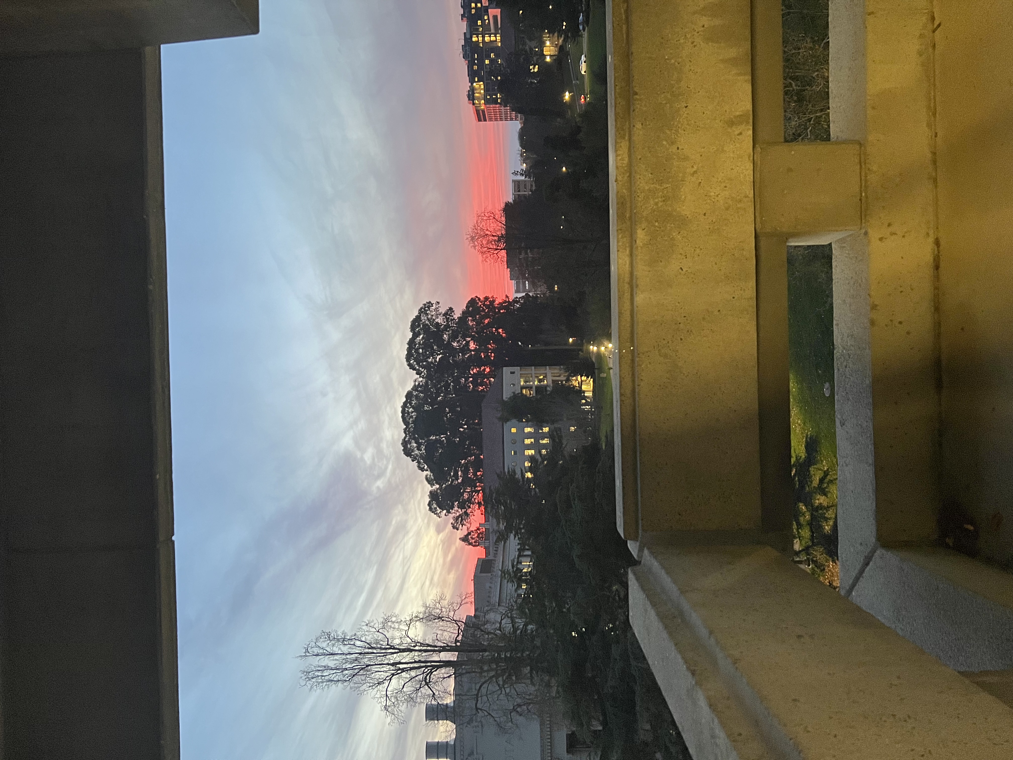
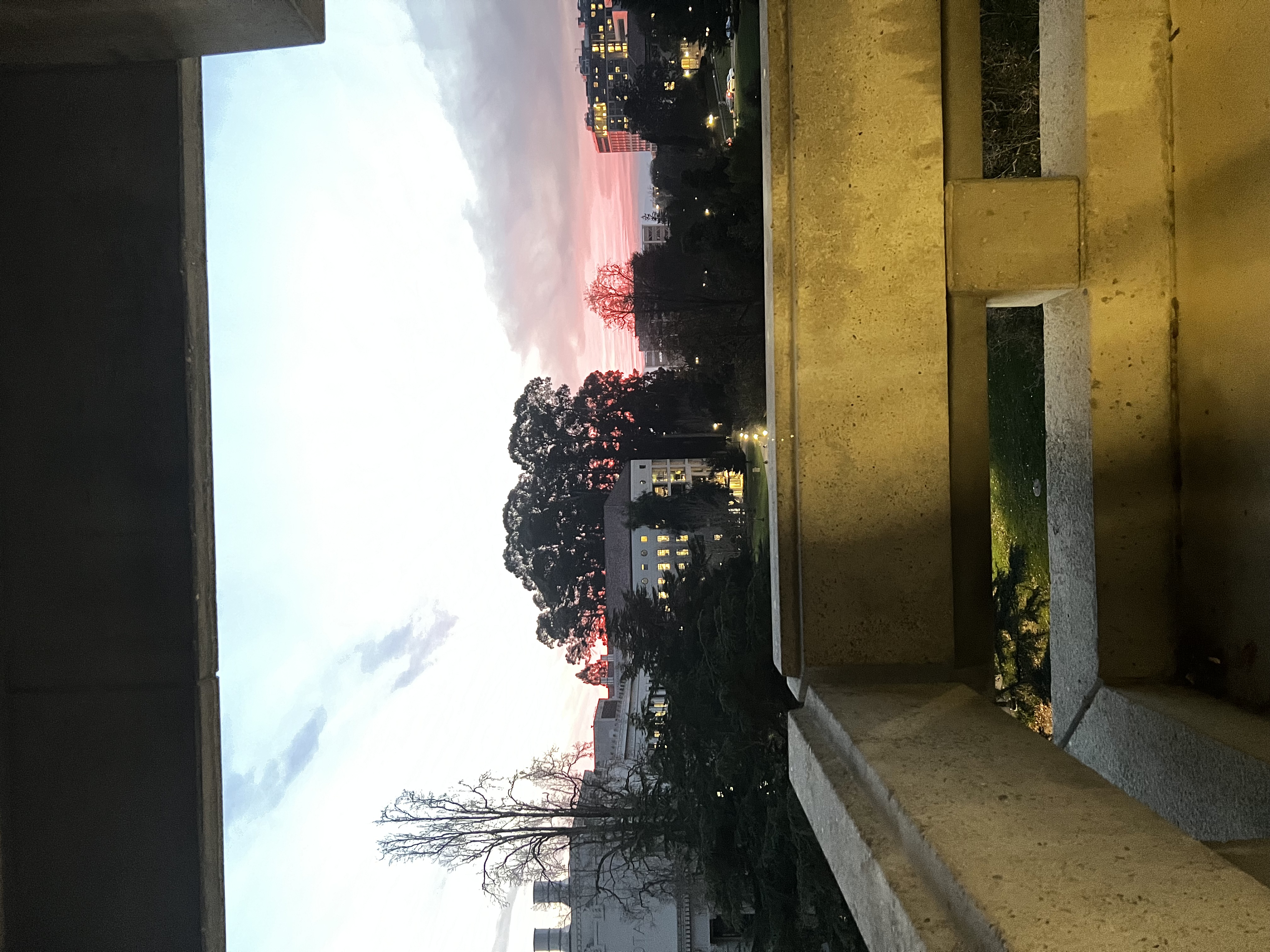
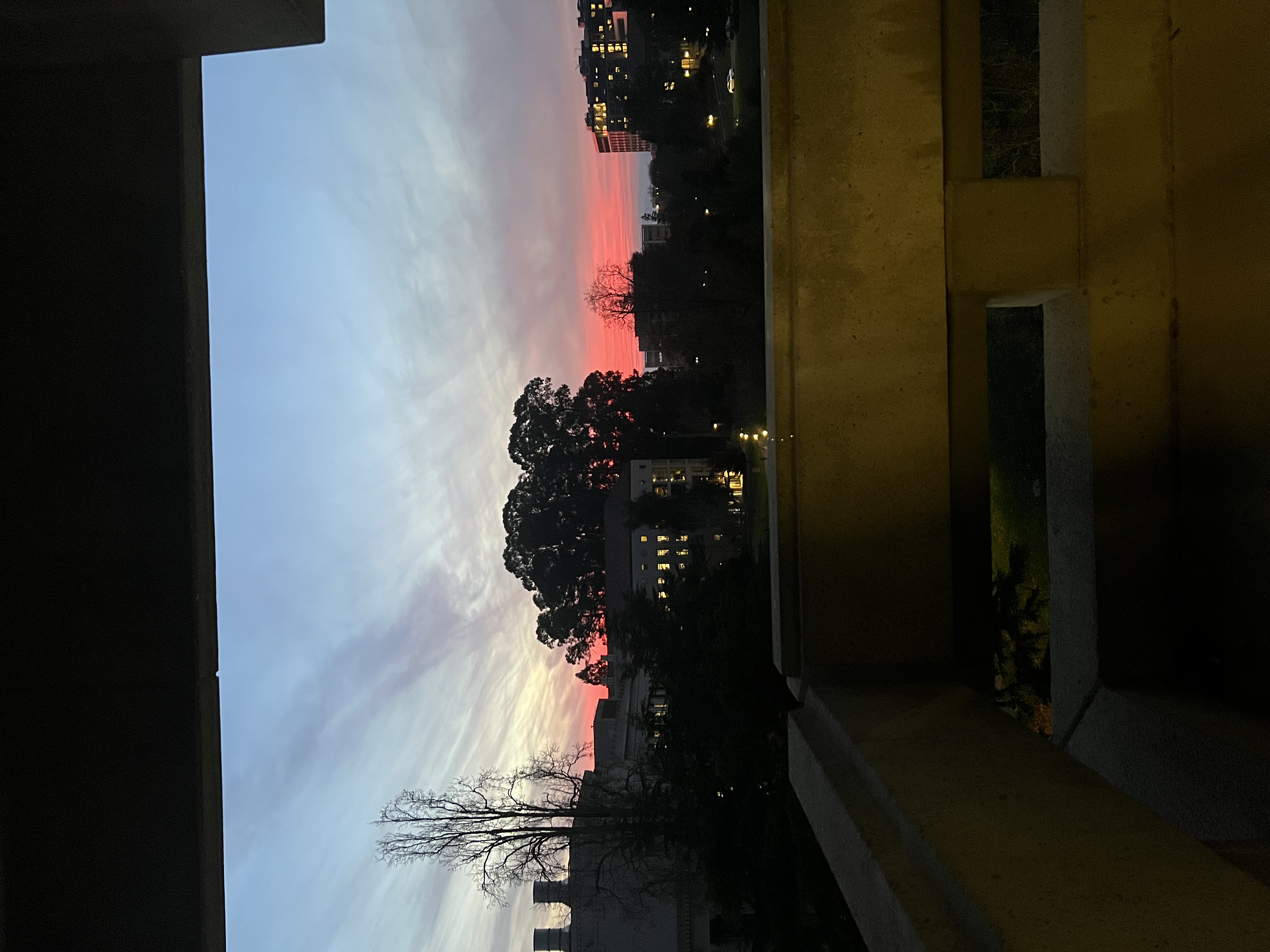
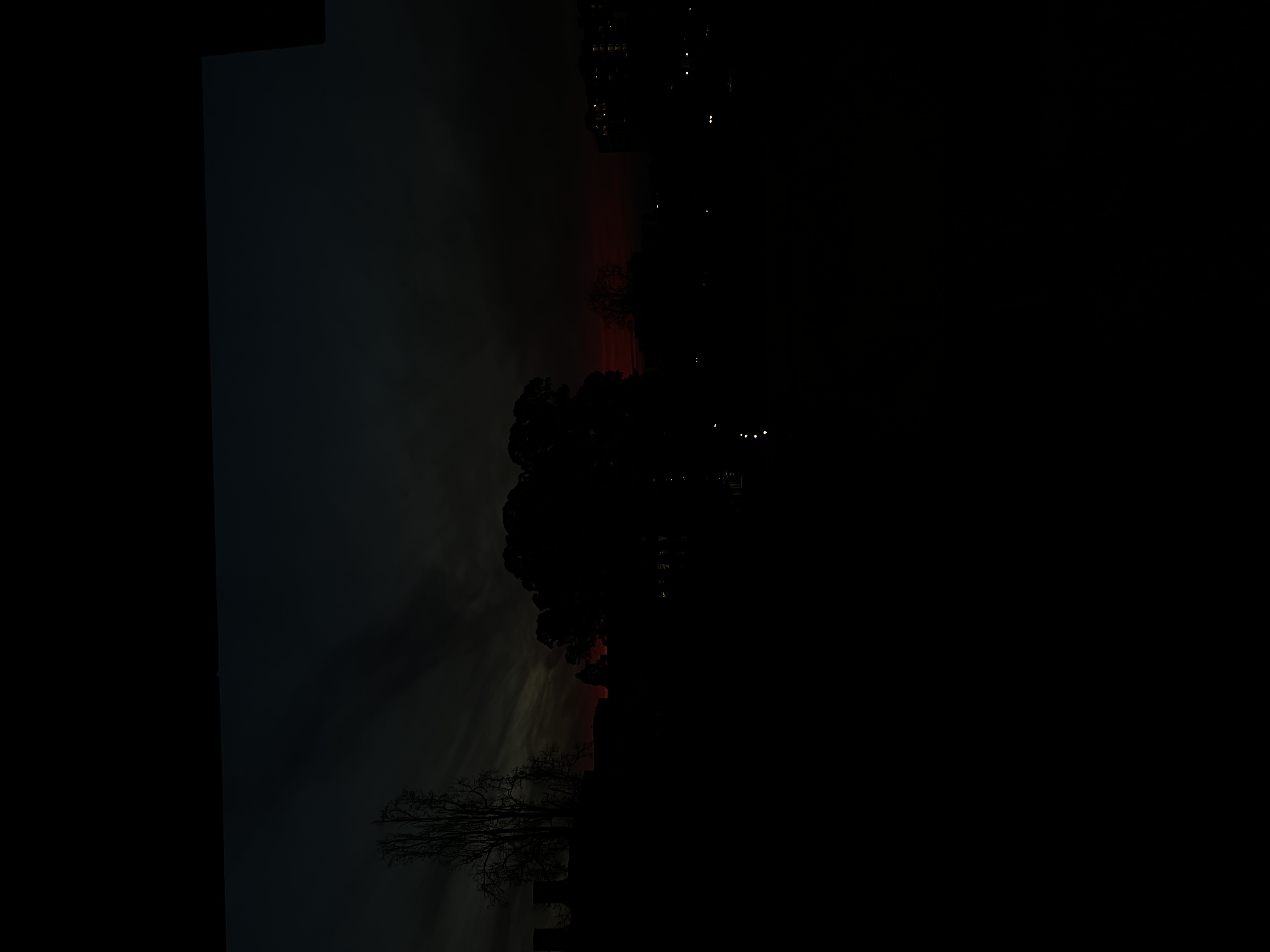
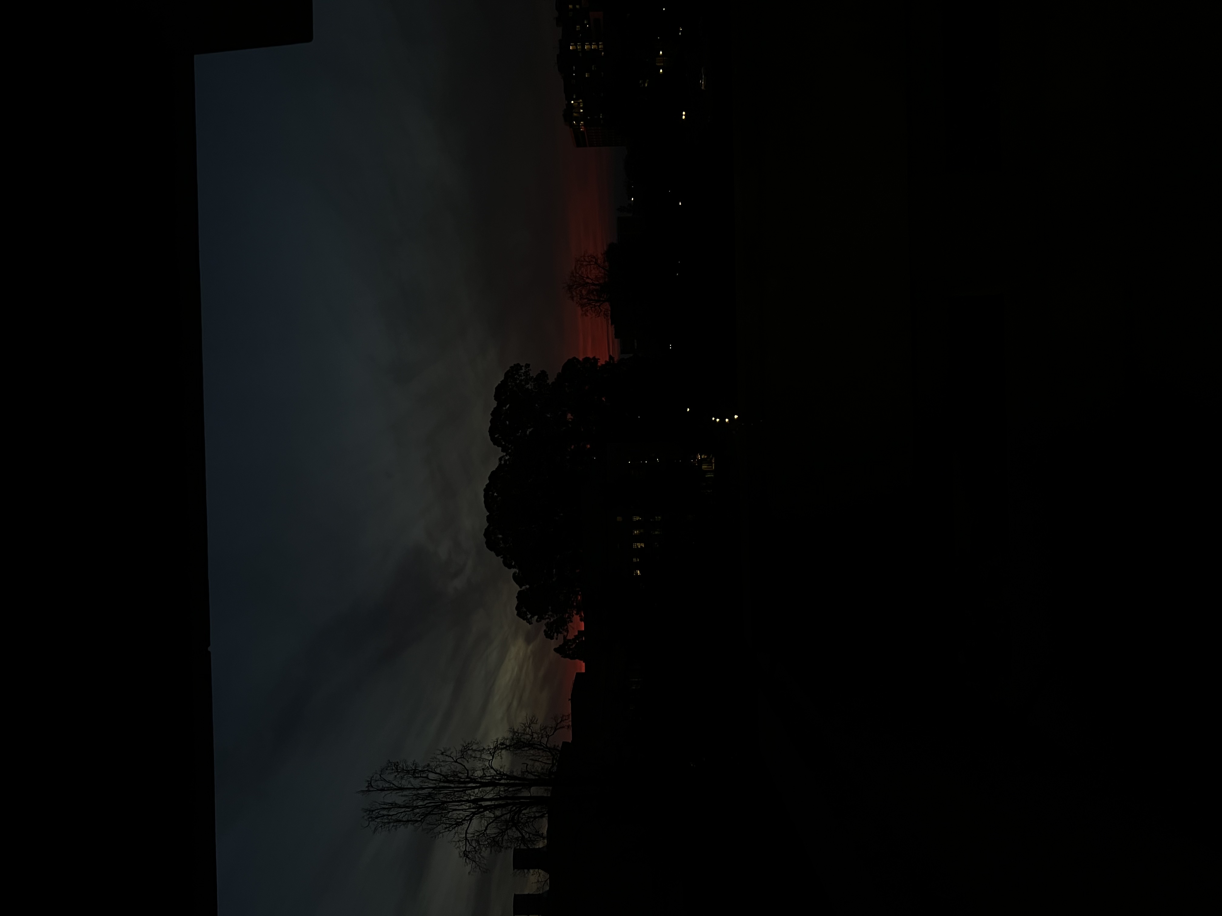
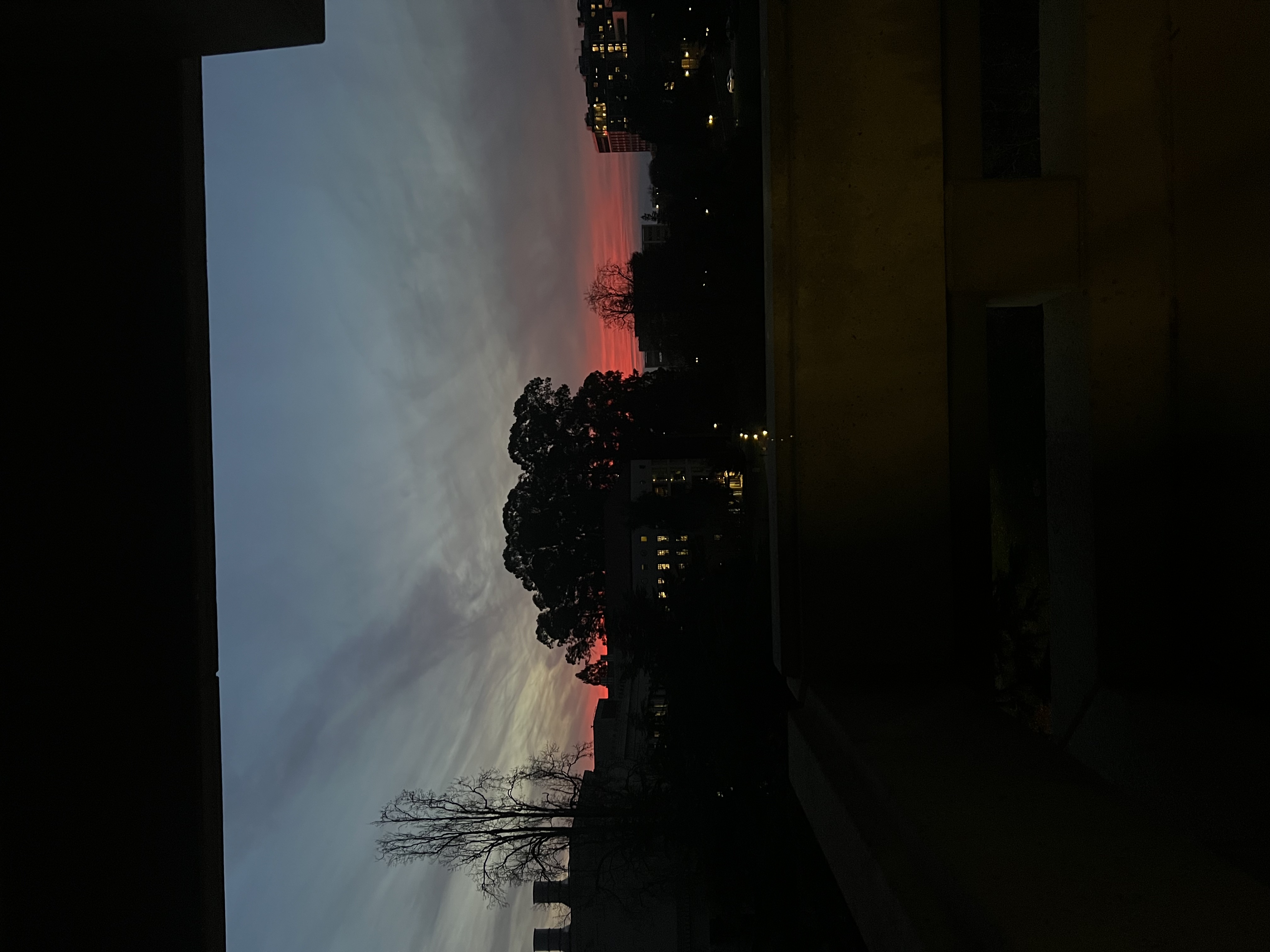
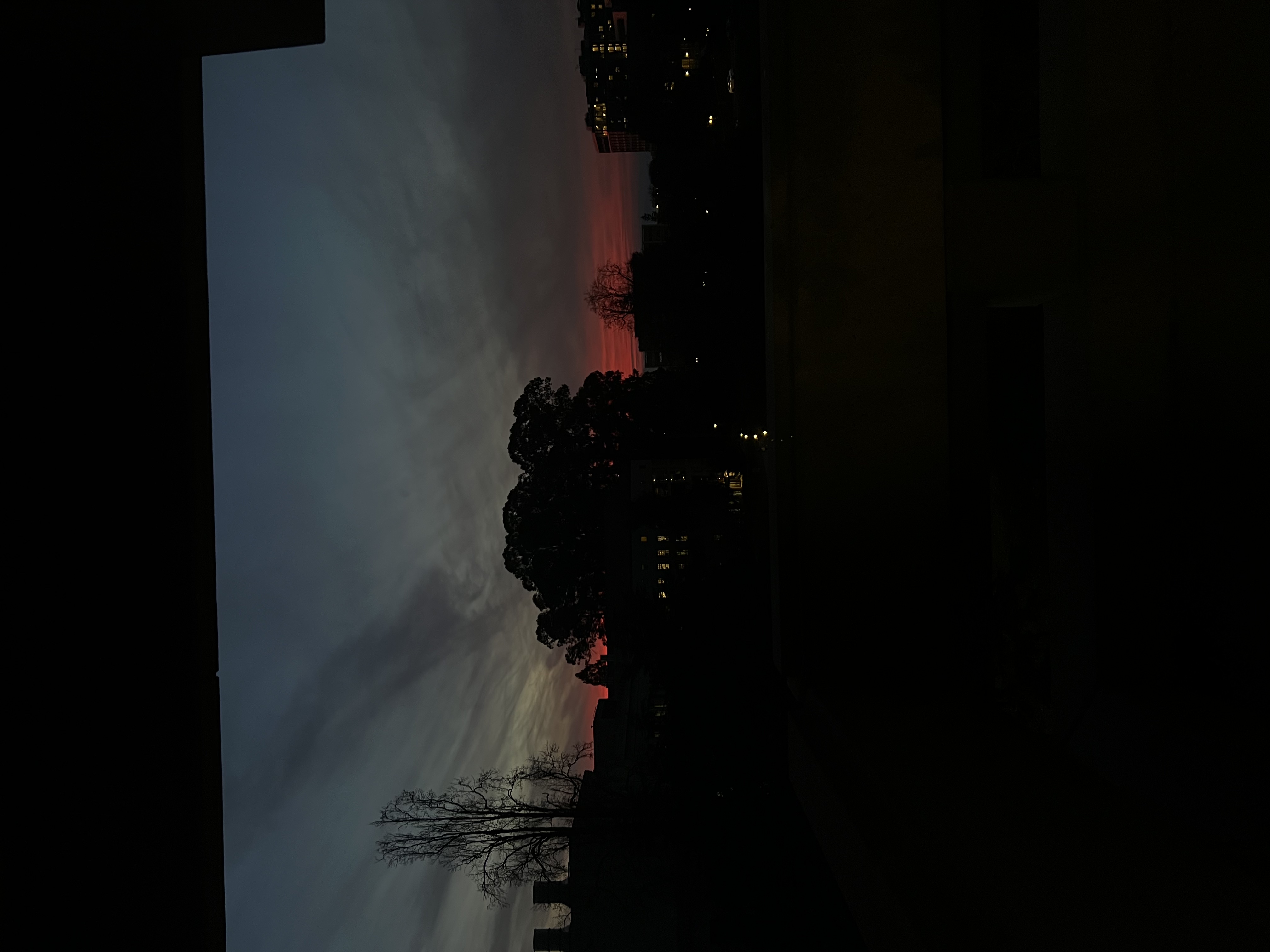
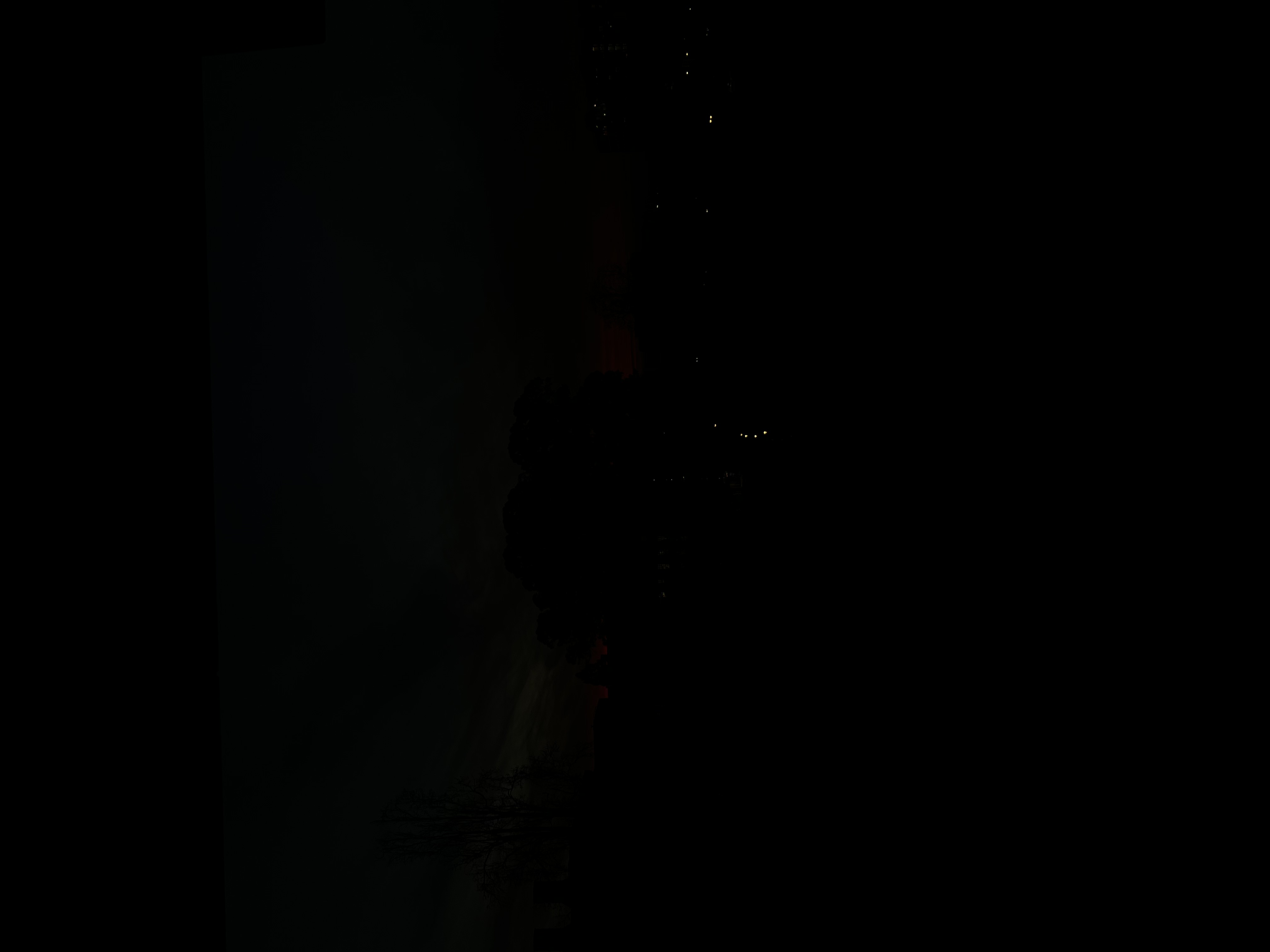
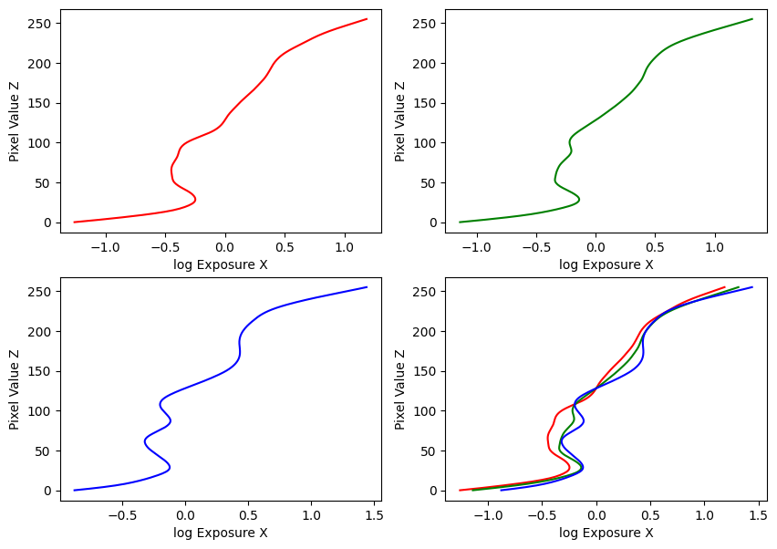
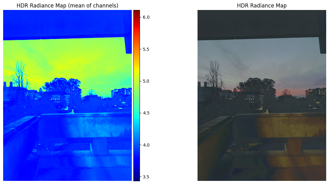
Estimated g and recovered radiance map for sunset
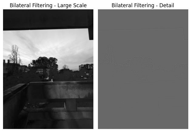
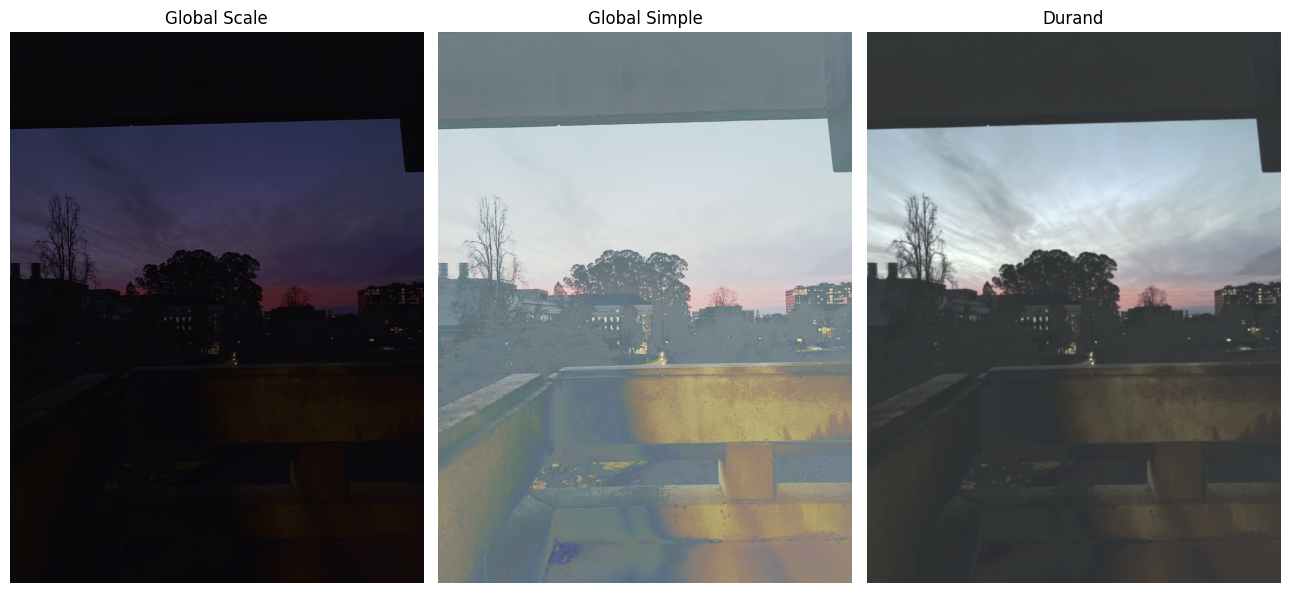
Bilateral filtering results and comparison of the three tone mapping methods for sunset
Image Set #3: Orange

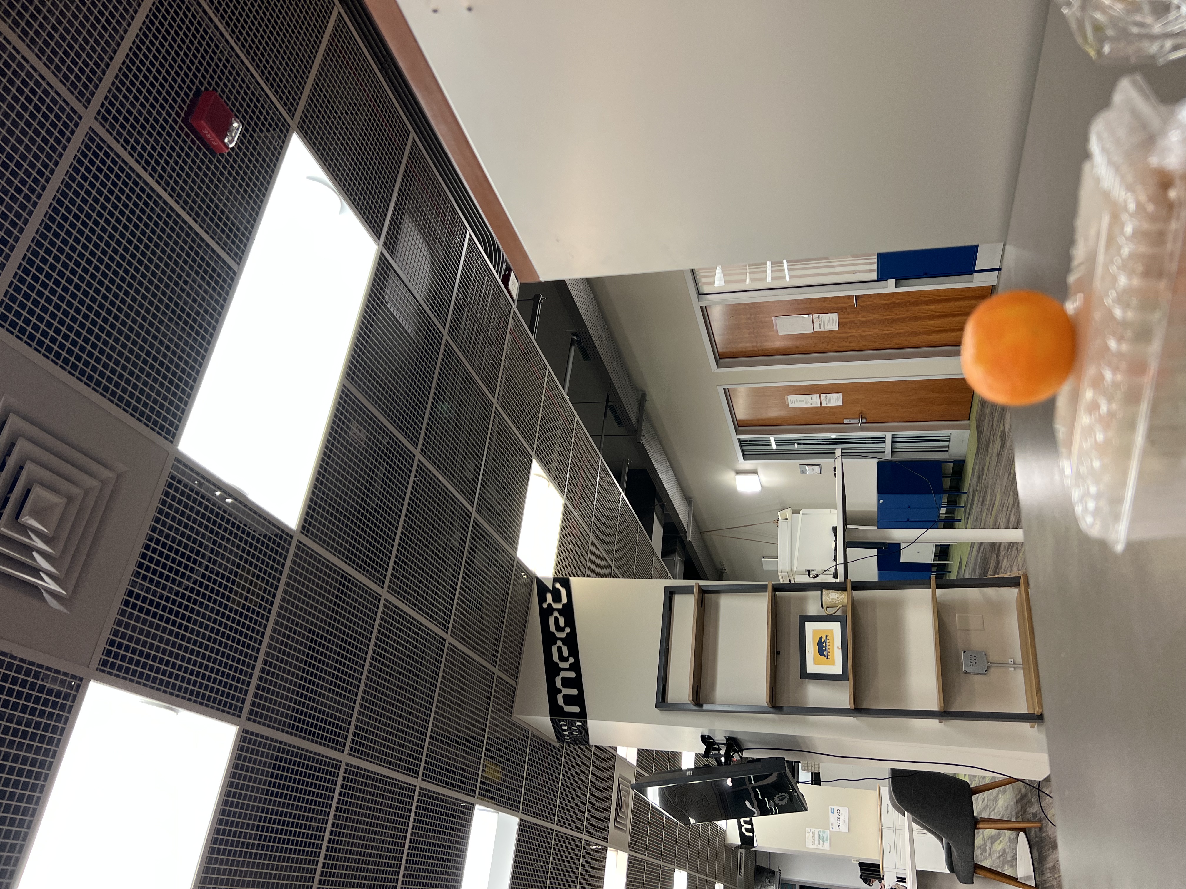
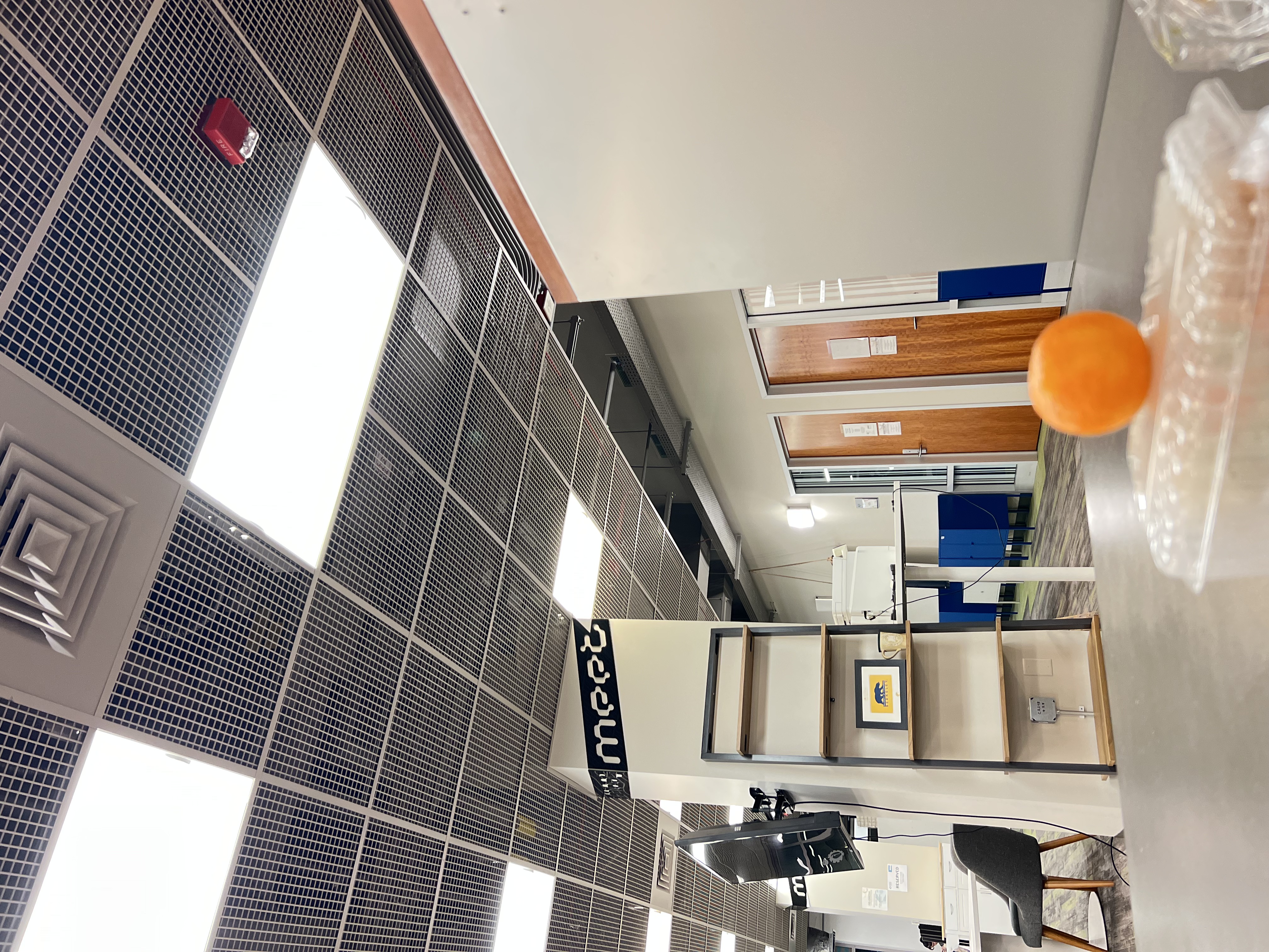
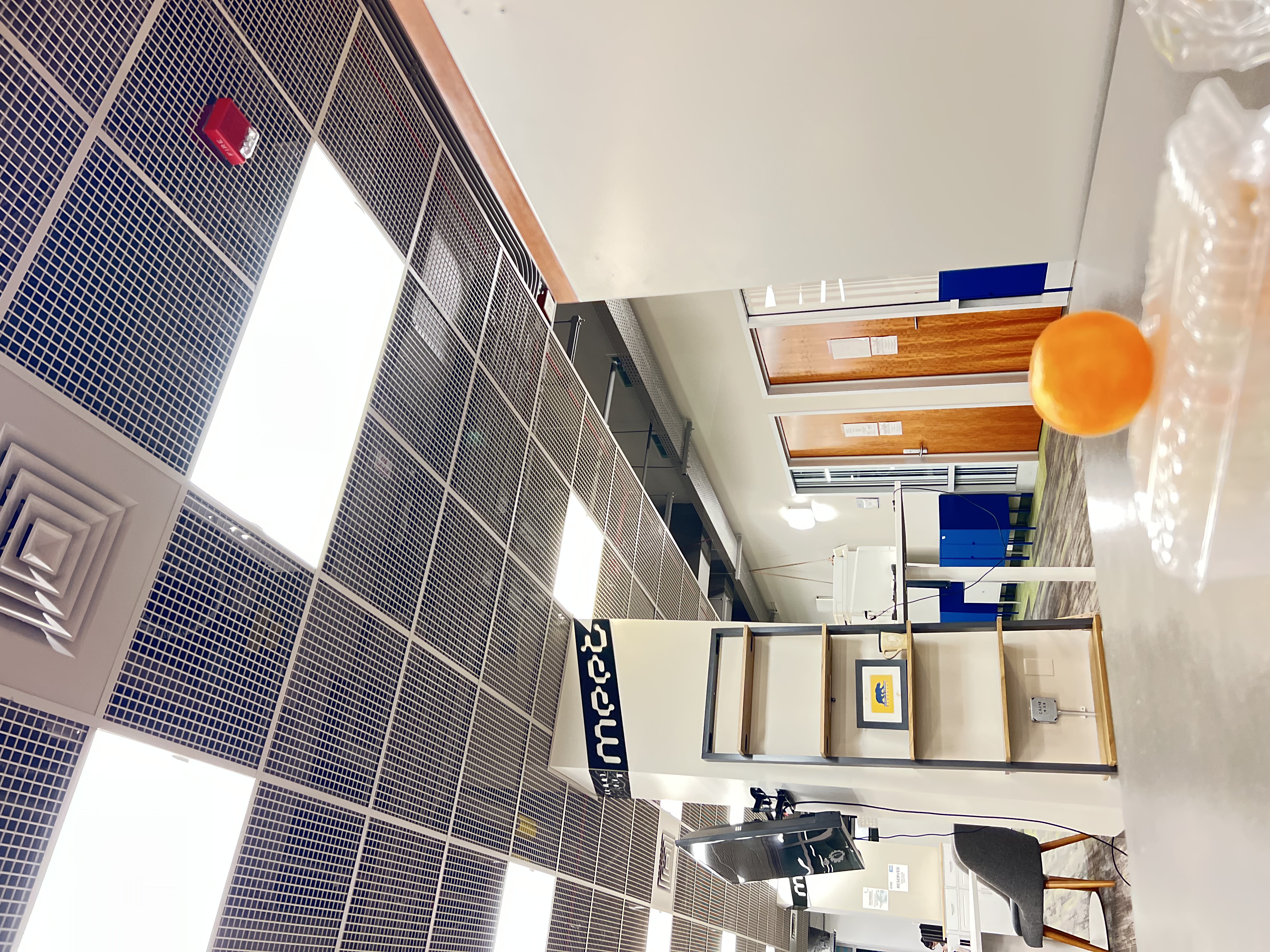
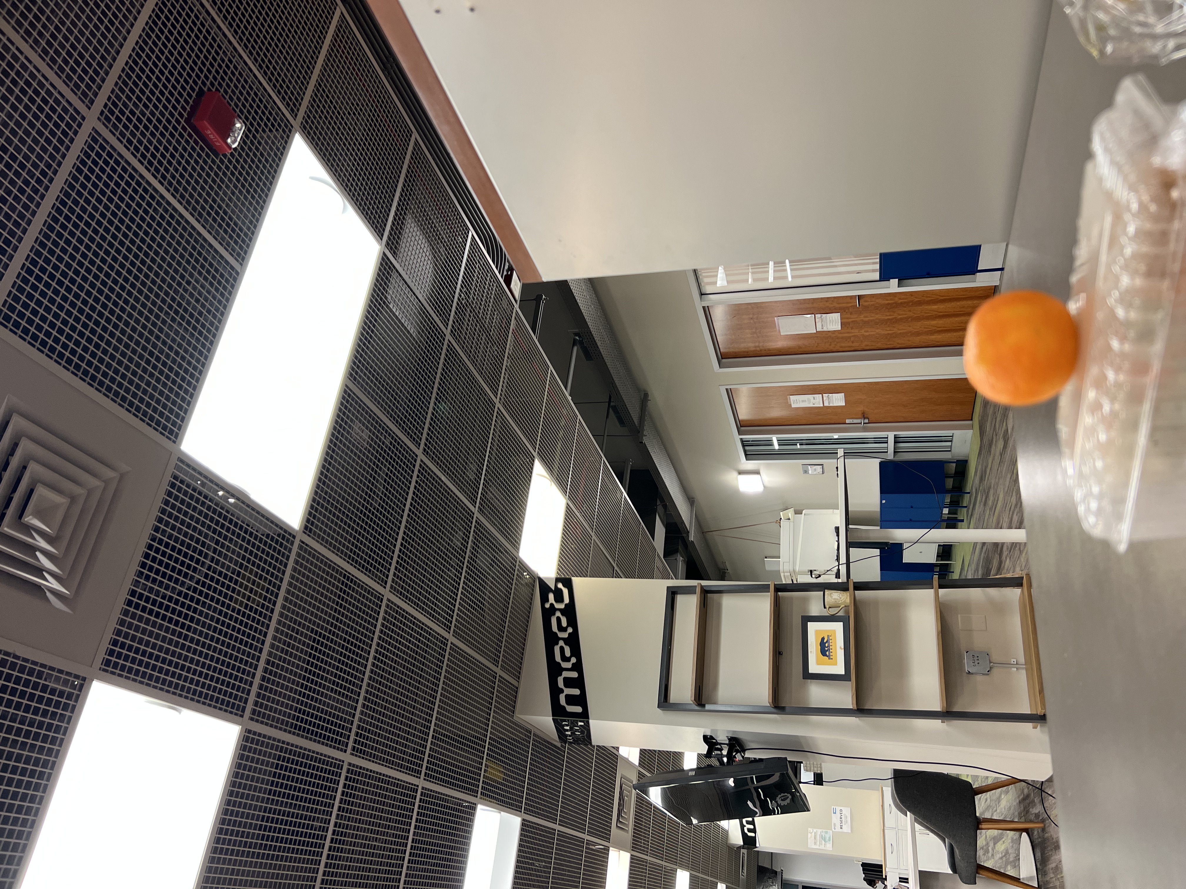
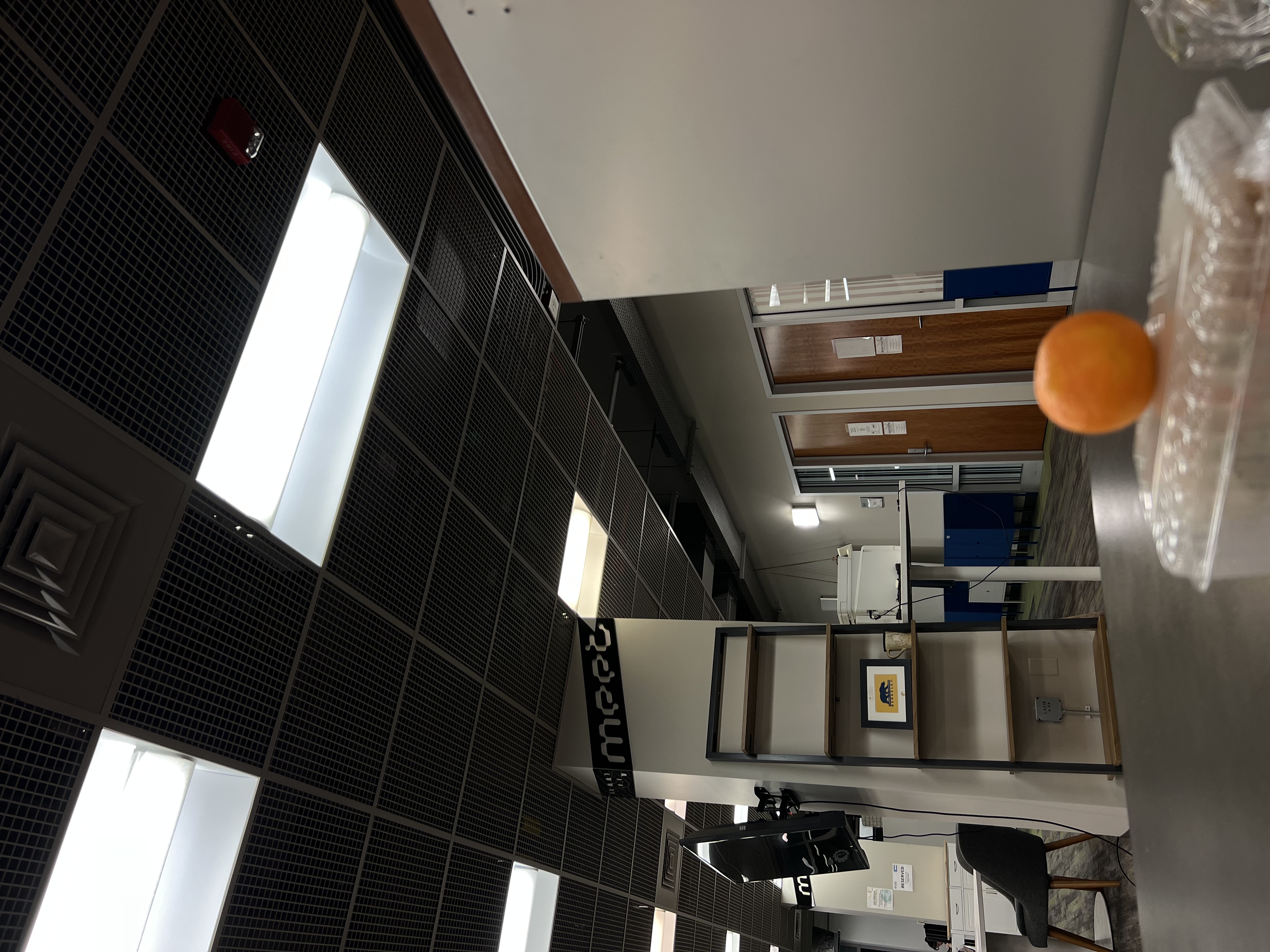
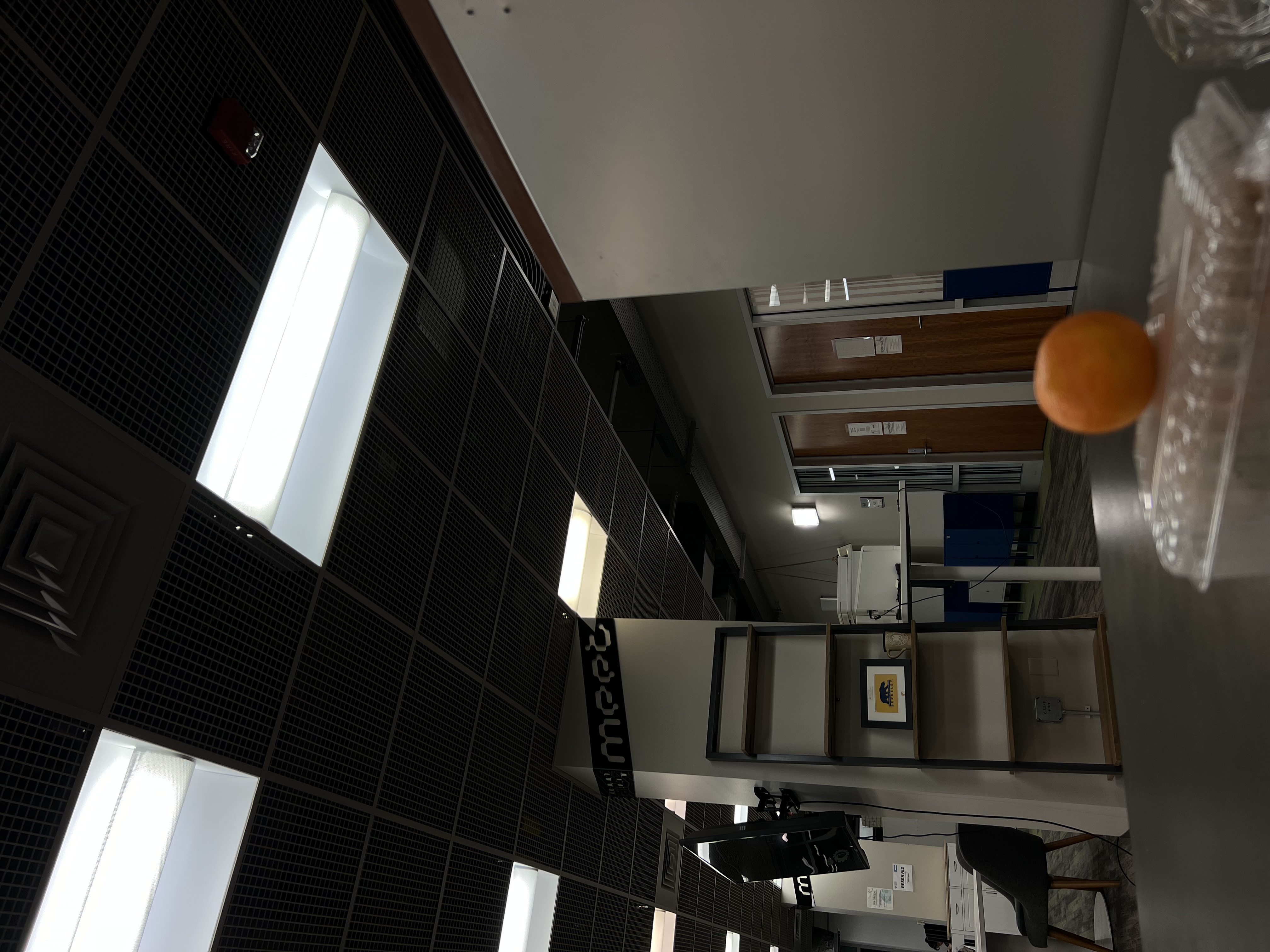
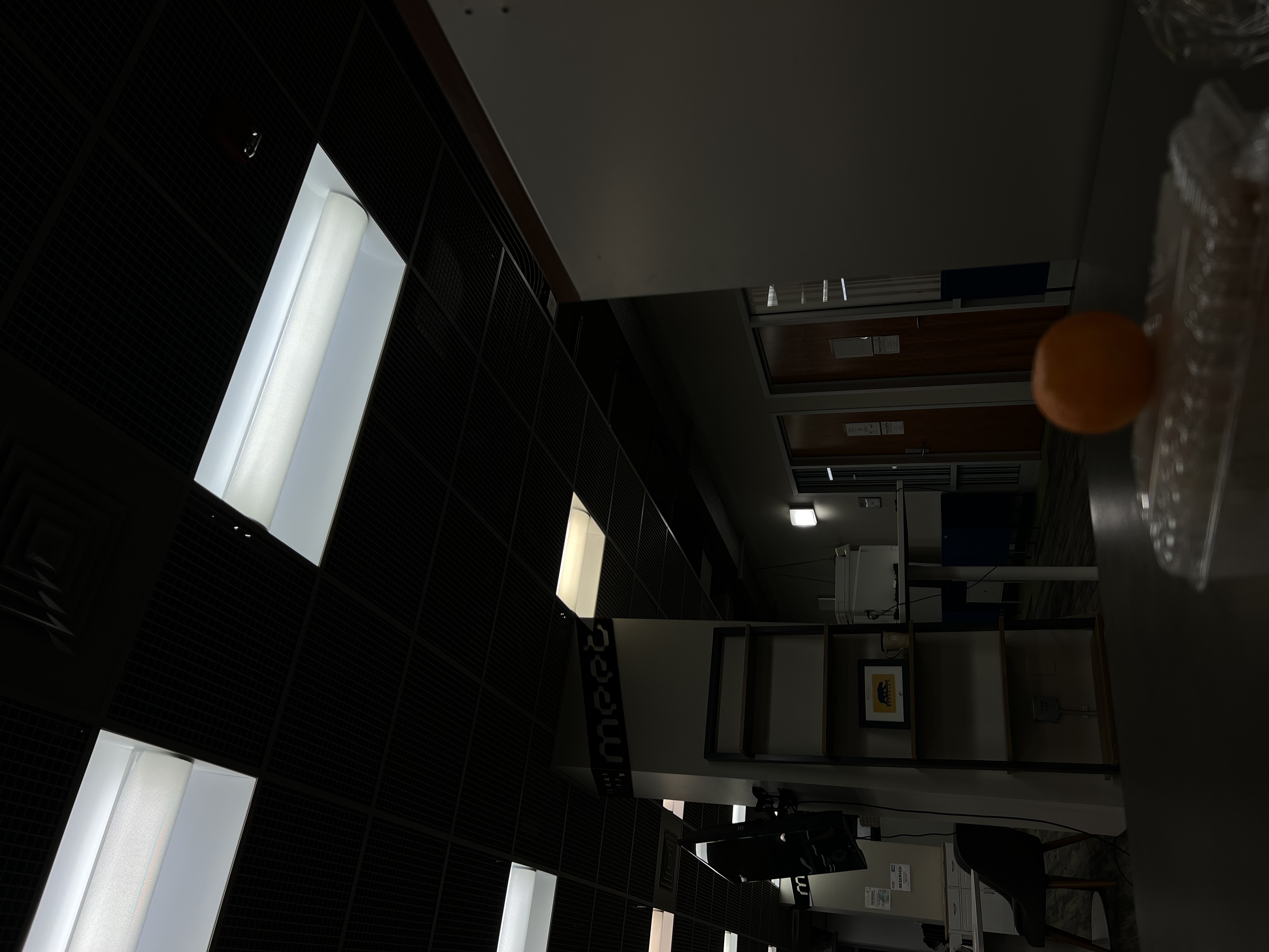
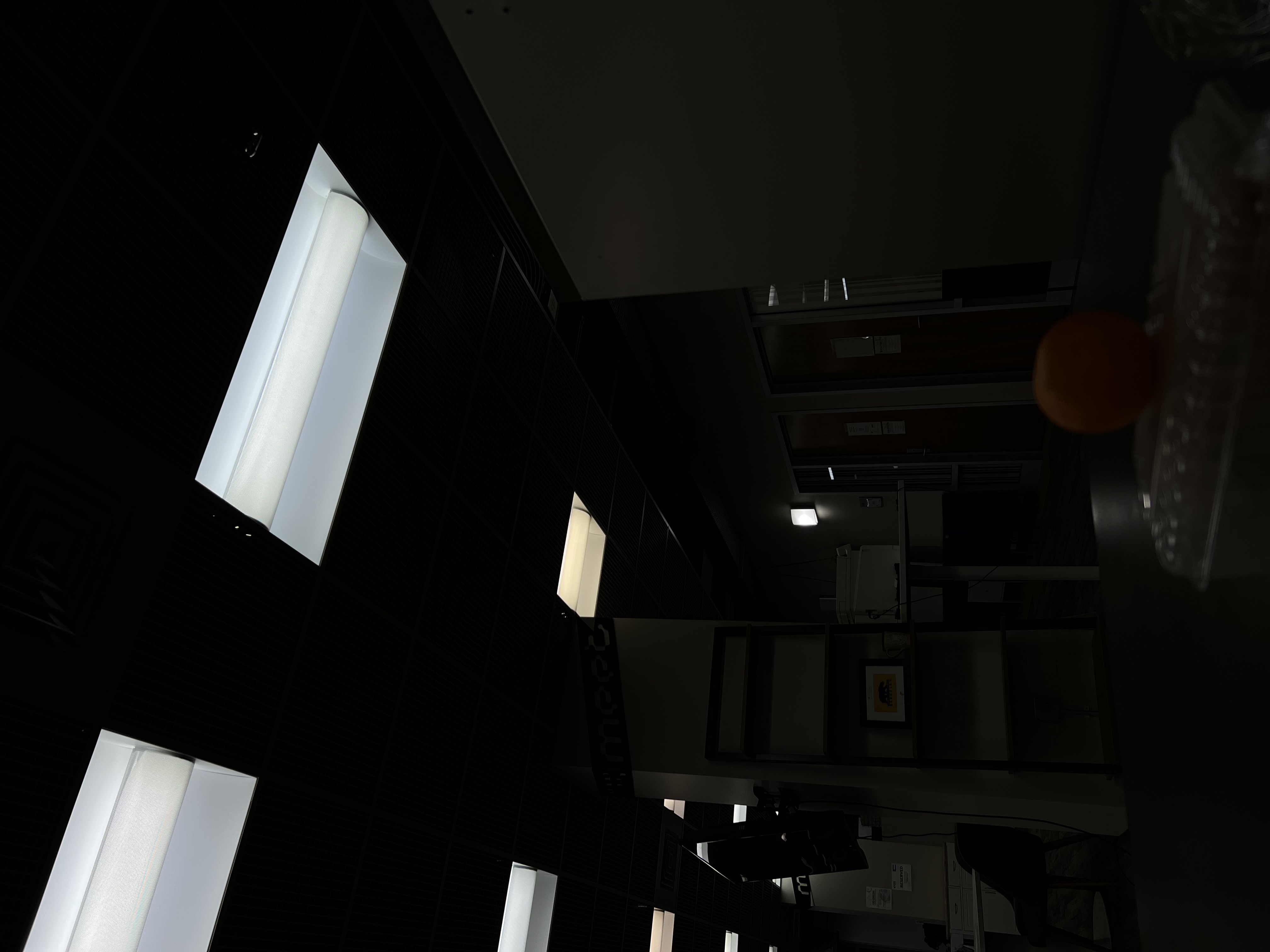
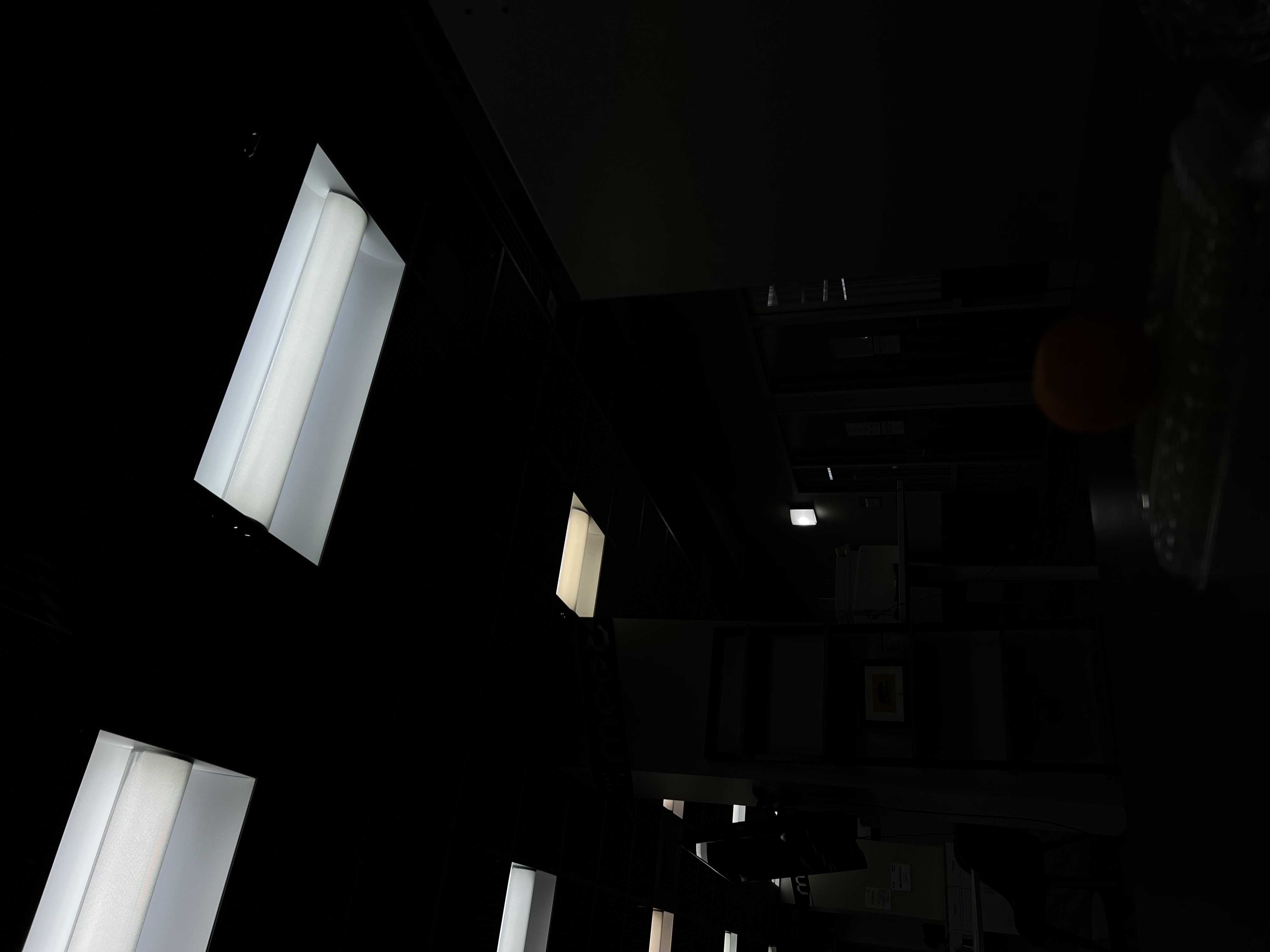
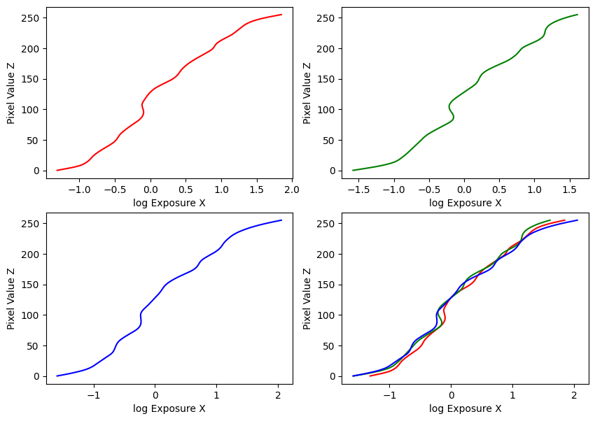
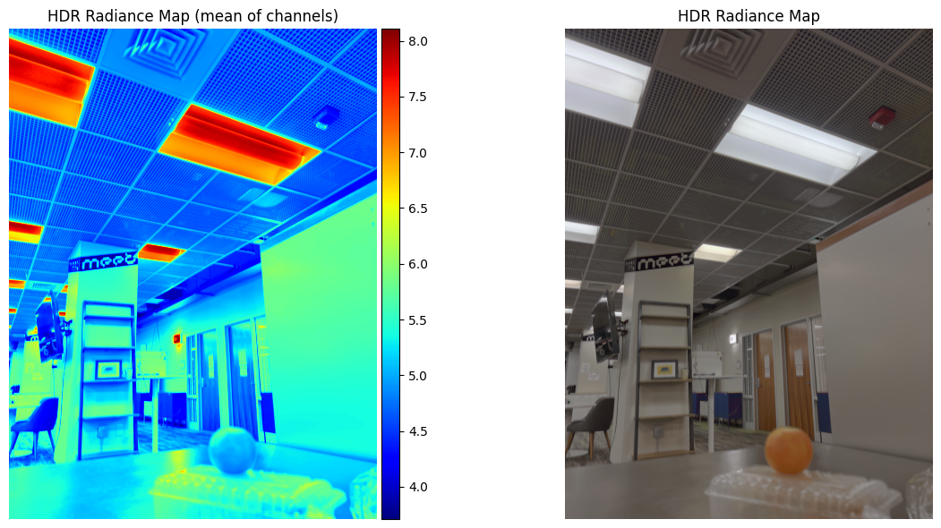
Estimated g and recovered radiance map for orange
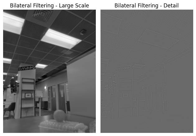
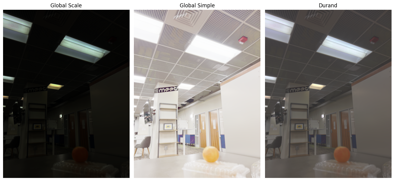
Bilateral filtering results and comparison of the three tone mapping methods for orange